Using a Kalman Filter to Rate NHL Players

Abstract  

For my research project, I wanted to combine my interest in hockey with my curiosity about data and math. I explored how a Kalman filter—a tool often used in engineering and statistics—could be applied to track NHL player performance during games. Instead of relying on end-of-season stats, which can sometimes be misleading, I built a system that updates each player’s rating shift by shift. It takes into account who was on the ice and the expected goal differential, giving a more accurate and real-time picture of how players are performing. This helps smooth out the effects of one unusually good or bad game and offers more meaningful insights. I hope this project not only helps fans and fantasy players better understand player impact but also shows how math and data science can be used to analyze the sports we love.  

Introduction  

In hockey, stats like goals and assists only tell part of the story. They don’t show what a player does without the puck or during defensive plays, which are just as important. That’s why analysts use a stat called expected goals (or xG), which measures how likely a shot is to become a goal based on things like where it was taken from and what kind of shot it was. While xG is more helpful than just counting goals, it still doesn’t tell you how much each individual player contributed to creating or preventing those chances. For my project, I wanted to build a better way to track player performance during games. I used a tool called a Kalman filter, which is great for situations that change quickly and randomly—just like in hockey. It allowed me to update each player’s rating shift by shift, giving a more accurate and real-time view of how they’re playing. 

Background on Kalman Filters  

The Kalman Filter, introduced by Rudolf E. Kálmán in 1960 [1], is widely used in control systems and aerospace to estimate hidden states over time from noisy measurements. Its ability to extract a “true” underlying value from uncertain data makes it well-suited for tracking player performance shift-by-shift in hockey, where single-game results can be noisy or misleading[3].  

At its core, the Kalman filter is a recursive algorithm that estimates the state of a system over time[2]. The “state” is something we want to track (like a player’s impact), and the filter uses a combination of past estimates and new observations to improve that estimate. 

The Kalman filter works by treating what we’re trying to measure—like a player’s skill— as something that exists but can’t be directly seen. Instead, we get noisy signals (like xG differential from shifts) that give us partial information. The Kalman filter then tries to  “guess” the true skill level over time by combining what it previously thought (the prediction) with the new noisy measurement (the update). 

Think of it like trying to track a car in fog. You can’t see it clearly, but you occasionally catch glimpses of it. Each glimpse is uncertain, but by combining all the glimpses and accounting for how much things could change or how noisy the observations are, you can make a better estimate of where the car is. That’s essentially what the Kalman filter does —but with math. To better understand why this works, we’ll break down the math and where it comes from. 

The Kalman filter is grounded in two core ideas: prediction and correction. It begins with a guess (called the prior) of a hidden variable—like player skill—and as new, imperfect data arrives, it updates that guess. The power of the filter lies in how it mathematically balances how much to trust the old guess versus the new data using probabilities. 

In mathematical terms, it minimizes the mean squared error of the estimate, assuming  Gaussian (bell-curve) noise. This gives it optimality in linear systems, which is why it’s used in everything from radar tracking and robotics to sports analytics.

The filter runs in a loop; every time new data comes in—in this case, each new shift in a game—and updates player ratings by combining what we already know with what just happened. 

The two main steps are called the prediction step and the update step. 

1. Prediction 

In this step, the filter predicts the next state of the system and how uncertain that prediction is. 

    •    State prediction: 

  xₖ₋₁ → x̂ₖ⁻ = x̂ₖ₋₁ 

    •    Uncertainty prediction: 

  Pₖ⁻ = Pₖ₋₁ + Q 

Here: 

    •    x̂ₖ⁻ is the predicted state estimate before seeing new data 

    •    Pₖ⁻ is the predicted uncertainty 

    •    Q is the process noise (random natural changes) 

2. Update 

Now the filter corrects its prediction using the actual observation from the new data.  

   •    Kalman Gain (how much we trust the new data): 

    Kₖ = Pₖ⁻ Hᵀ (H Pₖ⁻ Hᵀ + R)⁻¹ 

    •    Updated estimate:  x̂ₖ = x̂ₖ⁻ + Kₖ (zₖ − H x̂ₖ⁻) 

    •    Updated uncertainty:  Pₖ = (I − Kₖ H) Pₖ⁻

 where:

Zₖ: is the new observation (like xG_diff for a shift) 

   H:  is the matrix that maps the true state to what we can observe     

   R: is the measurement noise (how noisy our observation is) 

   Kₖ: is the Kalman Gain 

   x̂ₖ: is the updated estimate of the state 

   Pₖ: is the updated uncertainty 

These equations come from linear algebra and probability theory. The Kalman filter assumes the state evolves according to a linear model and that both the system and the measurement noise are Gaussian (bell curve-shaped) with known variances. 

The matrices Q and R represent how much randomness or noise we expect in our system and observations. If Q is high, we assume the underlying player skill changes a lot between shifts. If R is high, we assume our xG measurements are very noisy. Tuning these helps the model balance trust between past beliefs and new data. 

Where the Equations Come From  

The Kalman filter is based on the idea of minimizing uncertainty. It assumes that the current state (player rating) follows a simple rule: it either stays the same or changes slightly due to random factors. Observations (like xG_diff) are linked to the state through a matrix (H) and contain noise. The equations are derived by using Bayes’ Theorem to find the most likely state given the prior estimate and the new observation.  

In simple terms, each equation is designed to balance two forces:  

• “The prior (what we thought before this shift)”  
• “The measurement (what the shift data just told us)” 

The Kalman Gain (K) adjusts how much we move toward the new observation. If the data is noisy, we move less. If the prediction was way off, we move more. The math ensures this is done in the optimal way to reduce error. 

The update formula (posterior = prior + gain × error) is essentially a Bayesian update. It  answers: ‘Given what I used to believe and what I just observed, what’s the best new  belief?’ The Kalman gain determines how much we shift our belief, and this is computed based on how uncertain we are about both the prior (P) and the measurement (R).

Why the Kalman Filter Works  

The Kalman Filter works best in situations where you need to track something uncertain over time using noisy information. In hockey, a player’s true impact can’t be directly measured—we only see glimpses through stats like xG_diff. By combining the model’s previous belief with the new evidence from each shift, the Kalman Filter gives a smarter,  smoother estimate of how good each player really is. 

It also adjusts how much to “believe” each new data point based on how noisy it thinks that data is. If one shift has a weird result, the filter won’t overreact. But if lots of shifts show a consistent trend, it will gradually adapt the rating. 

Data and Setup  

I used public 5v5 shift data from Natural Stat Trick [5]. For each shift, I collected:  the list of offensive players and defensive players, and the expected goals differential (xG_diff)  

Each player was given a unique index number. Everyone started with a rating of 0, and I set small initial values for uncertainty and noise because I assumed performance doesn’t change too quickly. This setup allowed the model to slowly adapt as more shifts occurred.  

I used scalar values for the process noise and measurement noise. Specifically, Q=q⋅I and R=r, where I is the identity matrix. I manually tuned q and r to be small (e.g., q=0.01, r=0.1) to ensure stability and avoid overreacting to noisy shifts early in the season.  

Assumptions  

I assumed that the system is linear, noise is Gaussian with a zero mean, and that the covariance is known. 

Method: Using the Kalman Filter  

For every shift in the dataset, I built a vector H, where:  

 Offensive players = +1 

 Defensive players = –1 

This vector H∈R^1xn represents the players on the ice during a shift, where n is the total number of players in the dataset. Each element of H corresponds to a player’s index:  players on offense are set to +1, players on defense are set to –1, and all other values are  0. When we multiply H x X, we get the predicted xG differential for that shift, based on current ratings. 

Then I used the xG_diff from that shift as the observation (z) and ran the Kalman filter to update player ratings. The state vector x∈R^n holds the current rating of every player. Although only a small number of players are involved in any one shift, the Kalman Filter maintains this full vector across all players. The update only affects players present in the shift.  

Importantly, this means we’re not calculating each player’s contribution in isolation. The Kalman filter sees how the group of players on the ice performed together, then uses that to adjust everyone’s ratings just a little. So if a defensive player is consistently on the ice when their team allows fewer expected goals, their rating will slowly increase. This teamwork-based approach is one reason the filter gives more reliable ratings than just counting goals or points.  

How the Kalman Filter is applied to Player Ratings  

In each shift, I record the expected goals for and against (xG differential). Because multiple players are on the ice, the xG differential is influenced by everyone’s performance. I model the team-level xGD as a sum of the ratings of the skaters on the ice.  Using a Kalman Filter, I estimate and update each player’s rating over time. The filter updates a player’s performance estimate based on how the team performed while they were on the ice and how reliable that measurement is.

Let xk be a player’s latent rating at shift k, and zk be the observed xG differential for that shift. 

Prediction Step: 

x̂k | k − 1 = x̂k − 1| k − 1 

P_k|k−1 = P_k−1|k−1 + Q 

Update Step: 

K_{k =} P_k|k−1 

P_k|k−1 + R 

x̂k | k = x̂k | k − 1 + K_k(z_k − x̂_k|k−1) 

P_k|k = (1 − K_k)P_k|k−1

• x^k∣k−1: predicted rating before seeing the new shift 
• P: uncertainty in our estimate 
• Q: process noise (how much a player’s performance might vary) • R: measurement noise (uncertainty in xG) 
• K: Kalman Gain (how much we trust the new shift vs prior rating) 

I chose the Kalman Filter because it balances past performance with new shift data in a mathematically consistent way. Traditional models either rely too much on averages or overreact to single games. By using xG differential and updating shift by shift, this method smooths out variance while still responding to meaningful changes[6]. The assumptions I make include linear player contributions and Gaussian noise, which simplify computation while still producing stable ratings. 

For each shift, we follow this sequence:” 

1. Build matrix H, encoding who is on the ice (offense = +1, defense = –1).
2. Predict the expected xG_diff using current player ratings. 
3. Observe the actual xG_diff for that shift. 
4. Update each involved player’s rating based on the difference between prediction and observation. 
5. Repeat for every shift throughout the season. 

1. Prediction Step  

We first predict the current state before seeing the new data:  

x_prior = x 

This means we start by assuming the ratings from the last shift are still correct.  P_prior = P + Q 

 P is our current uncertainty (a covariance matrix), and Q is the extra uncertainty we add to account for performance possibly changing naturally. 

So this step gives us our best guess before seeing new data and tells us how confident we are in that guess.  

2. Update Step  

Now we use the new shift data to update our estimates:  

K = P_priorH^⊤S⁻¹

This tells us how uncertain we are about our prediction for the xG_diff on this shift.  

 H · P_prior · Hᵀ: how uncertainty in player ratings translates into uncertainty in xG_diff.  

 R: The noise in our observation of xG_diff.  

K = P_priorH^⊤S⁻¹ 

This is the Kalman Gain, which tells us how much to trust the new observation.  

Here, we assume the underlying ratings change slowly (low Q), and that the measurement (xG_diff) has moderate noise (R). The filter adapts depending on these values:  

 High R = less trust in new data, more weight on prior estimates  • High Q = belief that ratings can change quickly, so the model updates faster  

x_updated = x_prior ^{+ K} ₍z − Hx^prior) 

This is the main update:   z is the actual xG_diff observed.  H · Xprior is what we expected the xG_diff to be, based on current ratings. The difference is the “error,” which we scale with K and use to update ratings.  

P_updated = (I − KH) P_prior

Finally, we reduce our uncertainty. After seeing new data, we’re more confident in our updated ratings.

How It All Comes Together  

For every shift, we loop through the following sequence:  

1. Predict ratings and uncertainty 
2. Observe actual xG_diff 
3. Compare prediction to reality 
4. Update ratings and reduce uncertainty 

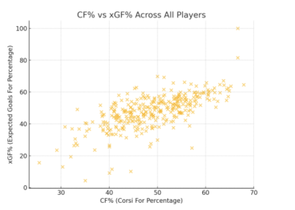
This repeats for every shift in the season, and over time, the ratings become smarter and more stable. Before applying the Kalman filter, it’s useful to see how shot share (CF%) compares to expected goal share (xGF%) across all players. 

Suppose a shift has three players: Player A, B, and C. A and B are offense, C is defense.

 The vector H=[1,1,−1], and the observed xG differential z=0.3. If we assume that the prior ratings x=[0.1,0.1,−0.1]. The predicted xG is H⋅x=0.1+0.1+0.1=0.3, which matches the observation, so the update is small. However, if z=0.6, the Kalman Gain would increase the offensive ratings and penalize the defensive rating accordingly. This is how the model incrementally adjusts player values. 

This example shows how, over time, each player’s rating becomes a reflection of their repeated impact. A player who always ends up on the ice during good shifts will see their score rise—even if they’re not scoring themselves. 

This process also prevents overreaction. If a player has one really strong shift, their rating only adjusts slightly. But if they consistently influence the xG_diff over many shifts, the filter learns to trust that signal more. This is what gives Kalman ratings their strength— they balance recency with consistency. 

Experiments and Results  

I ran this model on a full NHL season of shift-by-shift data[4]. As the season went on, each player’s rating changed depending on how much they helped or hurt the expected goals during shifts.  This yielded  the following observations:

 Players who weren’t big scorers still rated highly because they consistently created chances or prevented goals.  Players with big goal totals but poor defensive play sometimes ranked lower. Finally, the ratings were more stable than raw xG—less noise, fewer random spikes.  

 For example, Matty Beniers rated higher than expected due to consistent defensive contributions despite modest goal totals, while Patrick Kane had a lower rating due to poor xG_diff when on the ice, even though he scored often. 

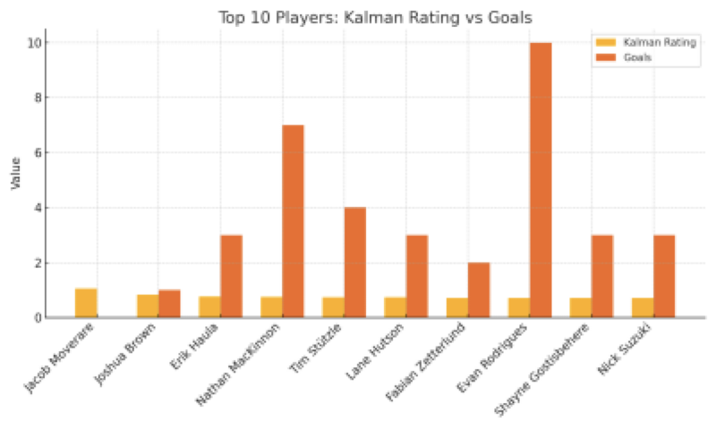
As shown in Figure 2 below, some players with strong overall performance (based on xGF%) ranked highly in the Kalman model even if they didn’t lead in goals.. This demonstrates how the model can highlight impactful players who may not lead in traditional scoring stats.  

Implications  

This type of model has real potential:   NHL teams could use it to find undervalued players or make smarter trade decisions.  Scouts could see who consistently impacts the game beyond goals. Fantasy hockey tools or betting models could use it to get an edge.  The method could work in other sports, for example, basketball or soccer.  The filter could be improved by adding more features for example ice time, face-off zones, or goalie performance.  

Conclusion  

Kalman filters offer a powerful, more balanced way to rate players. They combine old data with new information and avoid overreacting to one outlier shift. Compared to just looking at box scores, this model gives a fairer and more complete picture. This is a solid starting point—I didn’t include power play data or goalie stats— providing considerable potential for development. 

Code

The code is publicly  available in the repository below: https://github.com/Dimi Baguette/Kalman-Filter 

References  

[1]Kalman, R. E. (1960). A New Approach to Linear Filtering and Prediction Problems.  Journal of Basic Engineering, 82(1), 35–45.   https://doi.org/10.1115/1.3662552

[2]Welch, G., & Bishop, G. (1995). An Introduction to the Kalman Filter.  University of North Carolina at Chapel Hill.   https://www.cs.unc.edu/~welch/media/pdf/kalman_intro.pdf

[3]DraftKings Engineering. Kalman Filters for NBA Player Ratings.  https://www.draftkings.com/playbook/nba/kalman-filters-nba-player-ratings  

[4]GitHub Repository – Kalman Filter for NHL Player Ratings:   https://github.com/Dimi-Baguette/Kalman-Filter

[5]Natural Stat Trick – NHL Shift and Player Stats:   https://www.naturalstattrick.com

[6]Simon, D. (2006). Optimal State Estimation: Kalman, H Infinity, and Nonlinear Approaches.  Wiley Publishing.   https://onlinelibrary.wiley.com/doi/book/10.1002/0470045345

---