How Fair Are Fair Market Rents?

Abstract

Housing markets often defy the textbook principles of supply and demand. Economists expect that more housing supply should lower rents, but underlying affordability trends may suggest a more complicated reality. Using county-level data from the U.S. Department of Housing and Urban Development (OCC, 2014) from 2012 to 2025, this paper examines the relationship between unemployment, the construction of low-income housing, and fair market rents (FMRs). The analysis regresses unemployment rates against FMRs across multiple unit sizes and finds that there is a negative correlation between the two for all unit sizes (0-bedrooms to 4-bedrooms). It also tests whether greater low-income housing supply is associated with a reduction in rents; the results show a positive correlation between low-income units per 1,000 residents and FMRs, suggesting that affordable housing construction often follows rising rents rather than causing them to fall. However, when examining the share of low-income units within affordable housing projects, the correlation turns negative, indicating that the composition of affordable housing projects matters. These findings challenge the assumption that increasing supply alone improves affordability as a result of supply-side economics. The next step is to determine whether these trends have causal relationships, which will require expanding past HUD data to account for factors such as county-level political decisions, policing strategies, and domestic migration.

I. Introduction

Buying a home has long been considered a cornerstone of the American Dream, yet for  millions of Americans, it still remains out of reach. Even during periods of mass construction, affordability struggles persist, which raises questions regarding the factors that actually contribute to fair market rents (PD&R, 2025). Do areas with higher unemployment actually experience lower rents? And when states and towns invest in building low-income housing, does that added supply truly reduce rental costs? To answer questions like these, this paper focuses on fair market rents, the U.S. Department of Housing and Urban Development’s benchmark for affordability across counties in a given year.

Existing literature highlights the efforts of federal programs like LIHTC, which has financed over 2.4 million affordable units in the past 40 years (HUD, 2023). Yet scholars disagree on whether such efforts significantly improve affordability. Some argue that programs like LIHTC and inclusionary zoning stabilize house prices by expanding supply, but others believe that these policies have little impact on rents and can even correlate with increasing prices (Hamilton, 2019). To advance this debate, this paper examines how unemployment, the supply of low-income housing, and the composition of LIHTC projects correlate with fair market rents across U.S. counties and states.

This paper will be split into two main sections. First, I will evaluate the correlation between unemployment rates and fair market rents to measure if higher unemployment is associated with more affordability, since downturns in the labor market may reduce households’ ability to pay and push rents downward. This analysis will be done using county-year level data from HUD and will control for population and year. The second half of the paper will evaluate whether increases in the supply of affordable units are correlated with a decrease in Fair Market Rents. This analysis is significant as it will test the theory that more affordable units are associated with a decrease in prices; this section will use state-level data. Additionally, this section will evaluate how the percentage of affordable units within LIHTC projects correlates with fair market rents using the same state-year data. 

II. Fair Market Rents and Unemployment

A central question in housing affordability is whether local labor market conditions shape rental costs. A reasonable assumption to make would be that higher unemployment is associated with lower rents as weaker labor markets reduce household income and therefore constrain what renters are able to pay. This analysis tests that hypothesis using county-level data for fair market rents and unemployment rates since 2012. The FMR data is broken up by the number of bedrooms in a given unit ranging from 0-4.  

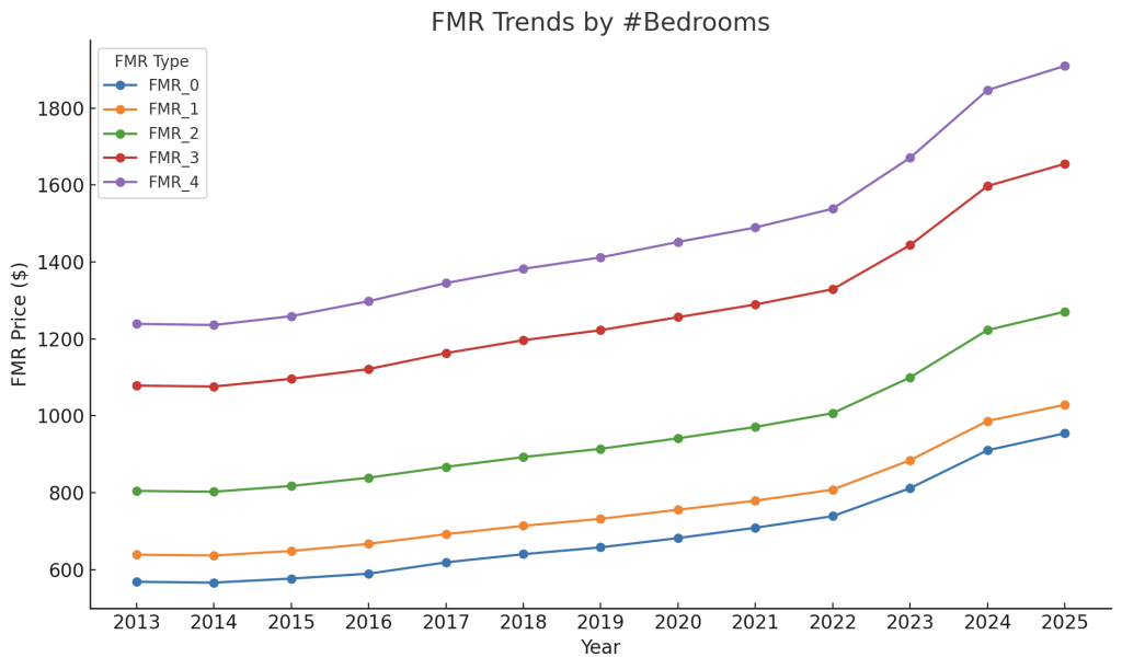
Figure 1 shows that FMRs have risen steadily across all unit sizes since 2013, with the greatest increases occurring after 2020. Specifically, there seems to be a gap between the fair market rents for 2-bedroom and 3-bedroom units suggesting that larger family-sized rentals have become less affordable at a faster rate.

Regressing this FMR data on unemployment rates attempts to understand how labor market conditions and affordability within a county relate to each other. After running multiple different regressions on FMRs and unemployment, the following results were outputted

Table 1 shows that when both county and year fixed effects are included, the relationship between unemployment and rents is weak, with high p-values, especially for two- , three- and four-bedroom units. Most coefficients fall close to zero and do not show a strong trend, with the exception of small positive values for studios and one-bedroom units. This result suggests that once both geographic differences and national trends are accounted for, unemployment alone does not explain much of the variation in rents. This outcome partially reflects the extent of the dataset: once both geographic differences and year-to-year shifts are absorbed by the model, little variation remains to be explained by unemployment alone.

Table 1: Regressions of Fair Market Rents on Unemployment

	0-Bedroom FMR	1-Bedroom FMR	2-Bedroom FMR	3-Bedroom FMR	4-Bedroom FMR
Unemployment Rate	0.998	0.881	0.018	-0.707	-0.584
p-value	0.007	0.027	0.969	0.248	0.452

Additionally, Appendix Table A.1 displays other regressions that were run on the data. Panel A of Appendix Table A.1 presents the results of a basic regression of rents on unemployment rates without any controls, the regressions show a consistently negative and highly significant correlation between unemployment and rents. A one percent increase in unemployment is associated with a drop of roughly $13.85 in the fair market rent for 0-bedroom apartments and $31.63 for 4-bedroom apartments. Additionally, FMRs decrease by greater intervals as the number of bedrooms increases. These results suggest that higher unemployment is linked with lower rents across all unit sizes.

Panel B of Appendix Table A.1: When county fixed effects are introduced, the negative relationship remains and grows stronger in magnitude. For example, a one percent increase in unemployment corresponds with declines of about $17.41 for 0-bedroom units and $36.21 for 4-bedroom units.The p-values remain at ~0.000, meaning that this is still a very strong relationship. This suggests that within the same county, periods of higher unemployment are consistently associated with lower rents.

Panel C of Appendix Table A.1: When year fixed effects are introduced, the correlation between unemployment and rents remains negative and statistically significant across all unit sizes. This indicates that even after accounting for national shocks, such as inflation or broad economic cycles, higher unemployment within counties is still correlated with lower rents.

Together, the regressions suggest a relatively consistent negative association between unemployment and fair market rents, specifically when looking at variation within counties or across years. When both county and year effects are controlled for, the relationship largely disappears, showing that some of the variation in rents is tied to structural differences across places and broad national trends. Overall, the results support the conclusion that unemployment and rent prices have a negative association.

III. Supply and Affordability

The concept that more supply leads to lower prices has guided federal and state investments in affordable housing for decades. Since the late 1980s, the Low Income Housing Tax Credit (LIHTC) program has been the central method for this effort, financing millions of units nationwide. By looking at annual LIHTC production, shown in Figure 2 below, I can see how policy and market conditions have shaped the pace of affordable housing construction over the past 40 years. 

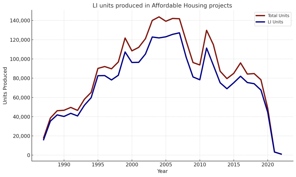
Figure 2 shows how the production of LI units has trended since the late 1980s. LIHTC production peaked in the early 2000s and in response to the 2008 crisis before declining in the 2010s. These shifts demonstrate how affordable housing construction responds to broader market and policy cycles rather than simply growing at a steady pace.

If adding affordable units truly decreases rents, states that build more low-income units (LI units) per 1,000 residents should have lower Fair Market Rents on average, given that other factors remain constant. It is important to calculate LI units given the population in the state in order to have a more applicable measurement for comparability. To test the hypothesis, FMRs were regressed on LI units per 1,000 residents using state–year data. The results are shown below:

Table 2 displays that when both state and year fixed effects are included, the relationship for 1-bedroom and 4-bedroom units is positive and significant for all unit sizes. These results show that even after accounting for state-specific characteristics and nationwide trends over time, more LI units per 1,000 residents continue to be correlated with higher FMRs. The data suggests that affordable housing is often added in response to rising rents rather than as a driver of lower rents.

Table 2: Regressions of Fair Market Rents on Low Income Units per 1,000 Residents

	0-Bedroom FMR	1-Bedroom FMR	2-Bedroom FMR	3-Bedroom FMR	4-Bedroom FMR
LI Units per 1,000 residents	11.690	10.320	14.120	19.200	14.090
p-value	0.000	0.002	0.000	0.000	0.025

Additionally, Appendix Table A.2 displays other regressions that were run on the data. Panel A of Appendix Table A.2: Without any fixed effects, the regressions show a consistently positive and significant correlation between LI units per 1,000 residents and rents. An additional unit per 1,000 residents is associated with increases of roughly $19.26 in the fair market rent for 0-bedroom apartments and $35.15 for 4-bedroom apartments These results are surprising because it shows that states with more LI units tend to have higher average rents. This result invalidates the hypothesis; however, this model does not control for any variables like rents increasing over time

Panel B of Appendix Table A.2: When state fixed effects are introduced, there is still a positive correlation and low p-values signifying a significant result. For example, an additional LI unit per 1,000 residents corresponds with increases of about $84.92 for 0-bedroom units and $157.80 for 4-bedroom units, both of which are over four times the coefficient of the simple model results. These results suggest that within the same state, years with greater low income housing production are also years with higher FMRs. This is an important measurement as there are many differences in affordable housing supply from state to state as represented in Figure 3 below.

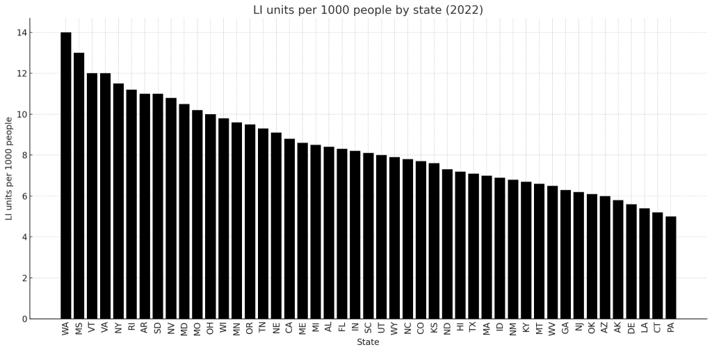
Figure 3 shows the disparity in affordable housing availability across the United States. States like Washington and Mississippi have more than twice the number of LI units per 1,000 residents compared to states such as Connecticut and Pennsylvania.

Panel C of Appendix Table A.2: When year fixed effects are introduced, the correlation between LI units per 1,000 residents and rents stays positive and significant across all unit sizes. This suggests that even after accounting for trends over time such as inflation, shifts in construction costs, etc., higher LI units per 1,000 residents within states are still associated with higher fair market rents. 

Beyond how many LIHTC units get built, the composition within each project matters: some developments set aside a small share of homes as affordable, others nearly all. After running regressions of FMRs on the percent of affordable units within LIHTC projects, the following results were outputted:

Table 3 shows that when both state and year fixed effects are included, there is a positive association between FMRs and the percentage of affordable units within LIHTC projects across all unit sizes. However, because the p-values are consistently high, the regression indicates that the relationship between affordable units and rents is ultimately unclear.

Table 3: Regressions of Fair Market Rents on Low Income Unit % in LIHTC Projects

	0-Bedroom FMR	1-Bedroom FMR	2-Bedroom FMR	3-Bedroom FMR	4-Bedroom FMR
LI Unit %	352	373	463	510	298
p-value	0.050	0.051	0.041	0.095	0.414

Additionally, Appendix Table A.3 displays other regressions that were run on the data. Panel A of Appendix Table A.3: Without any controls, the affordable unit percentage is negatively associated with FMRs. For example, a one percentage point increase in affordable units corresponds with a drop of about $171 for studios and $214 for two-bedroom units. These relationships are statistically significant for most unit sizes, however the p-value for three bedrooms and four-bedrooms make them insignificant. 

Panel B of Appendix Table A.3: When state fixed effects are introduced, the relationship flips direction. The coefficients flip, turning strongly positive and ranging from $1,130 for studios to $1,755 for four-bedroom units. This reversal suggests that within a given state, periods with more affordable unit concentration tend to coincide with higher rents. Again, the p-values for three and four bedroom apartments render them insignificant

Panel C of Appendix Table A.3: With year fixed effects, the relationship turns negative again. This pattern implies that after accounting for broad national shifts over time, higher affordable housing shares are associated with lower rents. This time, the relationship is significant for all fair market rent types.

As the coefficient fluctuates between positive and negative values and the p-values are higher for this data, I cannot conclude a statistically significant relationship between the percentage of affordable units  in LIHTC projects and FMRs.

IV. Conclusion

The results of this quantitative analysis highlight the true complexity of housing affordability in the United States. At the county level, unemployment and fair market rents have an inverse association: higher unemployment is consistently correlated with lower rents, and lower unemployment with higher rents. This negative correlation reflects the simple reality that when fewer households can afford rising prices, rents tend to fall. By contrast, state-level analysis of affordable housing supply produces a more surprising result. Instead of reducing rents, more low-income housing units per 1,000 residents are positively associated with higher FMRs, suggesting that construction often follows rising rents rather than driving them down. Lastly, when looking at the share of affordable units within LIHTC projects, the findings seem less clear. The coefficients change between positive and negative depending on which factors are controlled, and many large p-values weaken the statistical significance of the results.

While each state has pursued its own policies, the national patterns in this paper highlight the need to evaluate which approaches are most effective. Comparing state-level strategies and identifying the best models would be a logical next step toward solving the housing dilemma and creating real progress for real people. My hope for future research is to conduct high-quality, data-driven evaluations of state-level and county-level approaches to affordable housing, identifying patterns that reveal which methods are most effective in different contexts. This work could guide policymakers toward evidence-based solutions that expand access to affordable housing where it is needed most. The analysis would require extensive data collection, but the conclusions could provide strong evidence for policies that could actually improve affordability and restore the hope of the American Dream for millions of Americans.

V. Citations

Chan, Xiang Ying Estelle. The Impact of Affordable Housing on Housing Markets and Affordability. Massachusetts Institute of Technology, 2016. DSpace@MIT, https://dspace.mit.edu/handle/1721.1/107862

DeSilver, Drew. “A Look at the State of Affordable Housing in the U.S.” Pew Research Center, 25 Oct. 2024, https://www.pewresearch.org/short-reads/2024/10/25/a-look-at-the-state-of-affordable-housing-in-the-us/

Hamilton, Emily. Inclusionary Zoning Hurts More Than It Helps. Mercatus Center at George Mason University, Sept. 2019, www.mercatus.org/research/policy-briefs/inclusionary-zoning-hurts-more-it-helps

Office of the Comptroller of the Currency. Low-Income Housing Tax Credits: Affordable Housing Investment Opportunities for Banks. Community Developments Insights, Mar. 2014. U.S. Department of the Treasury, https://www.occ.gov/publications-and-resources/publications/community-affairs/community-developments-insights/pub-insights-mar-2014.pdf

U.S. Department of Housing and Urban Development. Federal Tools for Production and Preservation of Affordable Rental Housing. HUD User, 2023, https://www.huduser.gov/portal//portal/sites/default/files/pdf/Federal-Tools-for-Production-and-Preservation-of-Affordable-Rental-Housing.pdf

Wang, Ruoniu. Inclusionary Housing in the United States: Prevalence, Practices, and Production in Local Jurisdictions as of 2019. Grounded Solutions Network, Jan. 2021, https://groundedsolutions.org/wp-content/uploads/2021-01/Inclusionary_Housing_US_v1_0.pdf

Appendix

Appendix Table A.1: More Regressions of Fair Market Rents on Unemployment

Panel A: Simple Model (No Fixed Effects)

	0-Bedroom FMR	1-Bedroom FMR	2-Bedroom FMR	3-Bedroom FMR	4-Bedroom FMR
Unemployment Rate	-13.85	-15.08	-20.03	-26.54	-31.63
p-value	0.000	0.000	0.000	0.000	0.000

Panel B: Fixed Effects (county only)

	0-Bedroom FMR	1-Bedroom FMR	2-Bedroom FMR	3-Bedroom FMR	4-Bedroom FMR
Unemployment Rate	-17.41	-17.61	-22.71	-29.84	-36.21
p-value	0.000	0.000	0.000	0.000	0.000

Panel C: Fixed Effects (year only)

	0-Bedroom FMR	1-Bedroom FMR	2-Bedroom FMR	3-Bedroom FMR	4-Bedroom FMR
Unemployment Rate	-5.78	-7.40	-10.76	-14.71	-16.92
p-value	0.000	0.000	0.000	0.000	0.000

Appendix Table A.2: More Regressions of Fair Market Rents on Low Income Units per 1,000 Residents

Panel A: No Fixed Effects

	0-Bedroom FMR	1-Bedroom FMR	2-Bedroom FMR	3-Bedroom FMR	4-Bedroom FMR
LI Units per 1,000 residents	19.260	19.070	20.120	25.820	35.150
p-value	0.000	0.000	0.000	0.000	0.000

Panel B: Fixed Effects (state only)

	0-Bedroom FMR	1-Bedroom FMR	2-Bedroom FMR	3-Bedroom FMR	4-Bedroom FMR
LI Units per 1,000 residents	84.920	86.010	106.900	137.400	157.800
p-value	0.000	0.000	0.000	0.000	0.000

Panel C: Fixed Effects (year only)

	0-Bedroom FMR	1-Bedroom FMR	2-Bedroom FMR	3-Bedroom FMR	4-Bedroom FMR
LI Units per 1,000 residents	18.270	18.040	18.800	24.050	33.080
p-value	0.000	0.000	0.000	0.000	0.000

Appendix Table A.3: More Regressions of Fair Market Rents on Low Income Unit % in LIHTC Projects

Panel A: Simple model (no fixed effects)

	0-Bedroom FMR	1-Bedroom FMR	2-Bedroom FMR	3-Bedroom FMR	4-Bedroom FMR
LI Unit %	-171	-198	-214	-195	-193
p-value	0.006	0.003	0.008	0.063	0.122

---