Optimizing the Prediction of Small Deflections for Steel Cantilever Beams with Finite Element Analysis and Deep Learning

Author: Samarth Sethi
Mentor: Dr. Nikolaos Bouklas
Palo Alto Senior High School

Abstract

Surrounding literature around cantilever beams emphasize large deflection cases, where beam theory becomes geometrically non-linear and difficult to define analytically. As such, artificial neural networks (ANNs) are an established alternative method for predicting deflection, often being compared to finite element models for testing accuracy. While it seems prudent to reduce loss through utilizing only true beam geometries as the training data, our analysis reveals that appending dimensions outside the domain of beams can improve model fitting and return robust predictions. Extending the standard equation for bending stiffness (EI), the Euler-Bernoulli formula has been widely used as an analytical means of differentiating cantilever beam loads with respect to length in order to compute deflection along a certain axis. To avoid the mathematical complexity, we manually collected data on various true and non-true beam dimensions (length, width, and height), recording the deflection of the structures along the Z-axis with Autodesk Fusion’s Static Stress simulation software. As a substitute for differentiation, we trained MATLAB’s Feed Forward Neural Network and a Multi-Layer Perceptron (MLP), both of which are parameterized to the Adam optimizer and activation functions like RELU. Our central focus is to precisely predict the deflection of beam-like structures along the vertical axis for small deflection and distributed load cases only, assigning the dimensions as inputs to the neural network model. In terms of boundary conditions, we followed the general consensus for beam displacement: fixed-free. To validate the predictions for each data entry, we not only have testing values from the Fusion simulation, but analytical solutions within a percent error of 0.5-10%.

For reference, a deflection greater than the magnitude of the length of the beam divided by 10 is considered large. Otherwise, the deflection is small and linear, with simpler analytical solutions. Second, a beam geometry is considered to be true if its width and height are an order of magnitude smaller than the length.

Introduction

1. The Finite Element Method

In essence, the finite element method (FEM) divides a solid structure into simple parts or domains, regarded as mesh elements, that approximate certain functions related to physics. The structure’s deflection from a specific force load is often computed through the differentiation of these functions across each element and conjoining node (Chaphalkar et al., 2015). FEM as a physics replication tool has been criticized due to its long computation time and lack of accuracy. Because finite element analysis requires fine meshes to strictly estimate the components of a solid body, simulations of larger structures exchange exhausting wait times for near perfect results (Wang et al., 2020). In a dataset of deflections greater than 10^-6 meters, mesh refinement in the finite element model reduced the average error by 1%, but contributed to a tenfold increase in computation cost (Sargent et al., 2022). FEM simulations apply generous assumptions about the boundary conditions of structures. Whereas one end of a computer-designed structure could be fixed in space, real-world physics experiments expose how even rigid supports have significant degrees of elasticity, causing unnoticed error (Chaphalkar et al., 2015). That said, the raw definition of finite element is an approximation of analytical solutions to partial differential equations and integral equations. Such calculations are then simplified through ordinary differential equations, which are solved by numerical integration (e.g. Euler’s method). Despite its accepted limitations, the finite element method has diverse applications in civil, mechanical, and aerospace engineering (Oladejo et al., 2018). Rather, finite element computation softwares, most notably ANSYS, are utilized for continuous beam structures (fixed on both ends) with low degrees of error, warranting them as “multi-environment” and “multi-structural” (Lam Thanh Quang et al., 21)

2. Neural Networks in the Context of Physics

When a beam structure experiences a large deflection, its geometric shape will distort during bending, a non-linear problem that makes deflection difficult to predict with precision. In the past 10 years, physicists have employed the Euler-Bernoulli relationship to create analytical solutions for beams with large deflections under uniform loads. The relatively modern introduction of one- to three-layer artificial neural networks (ANN) combines linear and sequential prediction models with non-linear activation functions, returning errors below 0.5% in relation to known standard equations for deflection (Tuan Ya et al., 2019). For linear situations, error is minimized by preventing deflections from reaching large quantities, as exact values can diverge from the analytical solution. In a finite element analysis, a beam was stretched 50 to 55 degrees beyond equilibrium in the vertical direction. Only in this range was the error between 1.55% and 2.42%, when compared with the results of a physical experiment comprising a clamp and weight on the ends of the beam (Sargent et al., 2022). Regardless of the precision of measuring equipment (e.g. transducers or accelerometers), experimental validation methods remain limited by external conditions. Molecular friction, damping from the velocity of the beam, and aerodynamic damping all remove kinetic energy from the system, such that beam deflections fall short of their intended analytical value (Mekalke & Sutar, 2016). Precautions must be taken for beams that assume non-linear geometry upon a force load. As the magnitude of the load rises, the force at the arm of the shear external force sustains a reduction rather than a linear increase, thereby decreasing vertical deflection. In these instances, high values of loads are necessary to receive meaningful deflections (Kocatürk et al., 2010). Interpreting physics concepts through computer software not only ensures that computed results agree with the manual calculations, but offer insight into defining both linear and non-linear beam theory beyond the constraints of physics (Kimiaeifar et al., 13).

3. Recent Experimentation

Several researchers have applied shared methods in predicting the deflection of cantilever beams to the most precise degree possible. Oladejo et al. (2018)’s analytical solutions incorporated equations with bending stiffness (the product of the young’s modulus and moment of inertia) in the denominator as well as a young’s modulus value of 200 GPa, both of which reflect similar features as our own setup. Their study examined the effect of a far-end point load on the beam’s displacement, asserting the relationship between mesh refinement and model accuracy we make ourselves (Oladejo et al., 2018). As an extension of Oladejo’s model and experiment, Samal & Rao (2016) implement a 10-node element mesh, while analyzing the deflection error of a uniformly distributed beam load in addition to a point load. Although the methodology for cross-validating the finite element method results with the analytical solutions remained constant, the percent error varied largely between 0.97% and 51.26% for the distributed load and between 0.5% and 26.4% for the point load (Samal & Rao, 2016). The explanation for why the distributed load returns a greater error than the point load in their model may be attributed to the computational bandwidth of the ANSYS software they used, a drawback we hope to improve through our own finite element and data collection processes. Now, Chaphalkar et al. (2015) follows suit with us and other structural engineering researchers in calibrating the finite element model to a cantilever beam with a young’s modulus of 210 GPa and a material of mild steel. Bolstering the credibility of our own methods, the dimensions of the beam analyzed included a length of 0.8 m, width of 0.050 m, and height of 0.006 m, in the range of our own beam iterations by an indistinguishable amount. However, as opposed to the maximum deflection, they recorded the experimental frequency of a fixed-free beam, verifying their finite element analysis with a simple procedure of tapping a lightweight beam and measuring the resulting oscillatory motion. Granted that amplitude is often proportional to frequency, and the boundary conditions are generalized for beam deflection problems (fixed-free), the percent error of the oscillation experiment being 5-7% should confirm the pertinency of FEM in the context of this paper. Another study from Mekalke & Sutar (2016) describing the frequency of beams’ elastic motion also had a target objective to predict the extrema of frequencies as a means of avoiding resonance, or damage to real-world beam structures. Thus, the maximum deflection was a major dependent variable in their ANSYS FEM simulation, in which they tested 15 beam geometries with 3 varying materials and the young’s modulus of 210 GPa we share. Designating the Euler-Bernoulli analytical solutions as their validation set, their most crucial finding concerned how the most damage occurs at the maximum amplitude, possibly linking Sargent et al. (2022)’s claim about large deflection errors to degradation of the beam system (Mekalke & Sutar, 2016). Lastly, Tuan Ya et al. (2019) offers a complementary baseline for our research, as their procedure contains explicit similarities. In probing the neural network, they split the data into a 7 : 1 training to testing ratio, while noting that the network with 3 hidden layers produces the most optimal accuracy. The standard deflection equation for cantilever beams (exempt of derivatives) is a replica, even though multiple variations of the formula exist depending on the load type. Considering that the final artificial neural network model achieved a percentage error between 0.08% and 0.43% for vertical deflections, it is suggested that we strive for a loss in or below this range (Tuan Ya et al., 2019).

Methodology

We recorded the length, width, height, and deflection of 36 unique cantilever beams, including an additional 36 separate structures that exhibit similar deflection properties as beams. The extrusion geometry was entirely unchanged, except for the dimensions of the extruded face and the horizontal depth of the beam. In establishing the parameters for our simulation, we considered the boundary conditions, loading values and distribution, and the material properties of the beams we designed. The analytical solutions calculated for deflection act primarily as a validation for the finite element results. In Fusion360, as is the expectation of finite element analysis, the simulation will not solve for the established conditions until a mesh is provided.

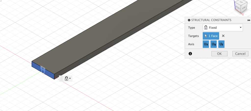
Autodesk Fusion provides a series of different boundary conditions (labeled as ‘Structural Constraints’ in the interface of the software), including but not limited to the standard “fixed” that can be applied to faces of the structure, a “pin” constraint that prevents movement in axial directions, and a “frictionless” condition that locks any movement normal to the surface. For the simulations we solved, we applied a “fixed” structural constraint to the far end of the beam, inhibiting degrees of freedom in all X, Y, and Z directions at the face. See below:

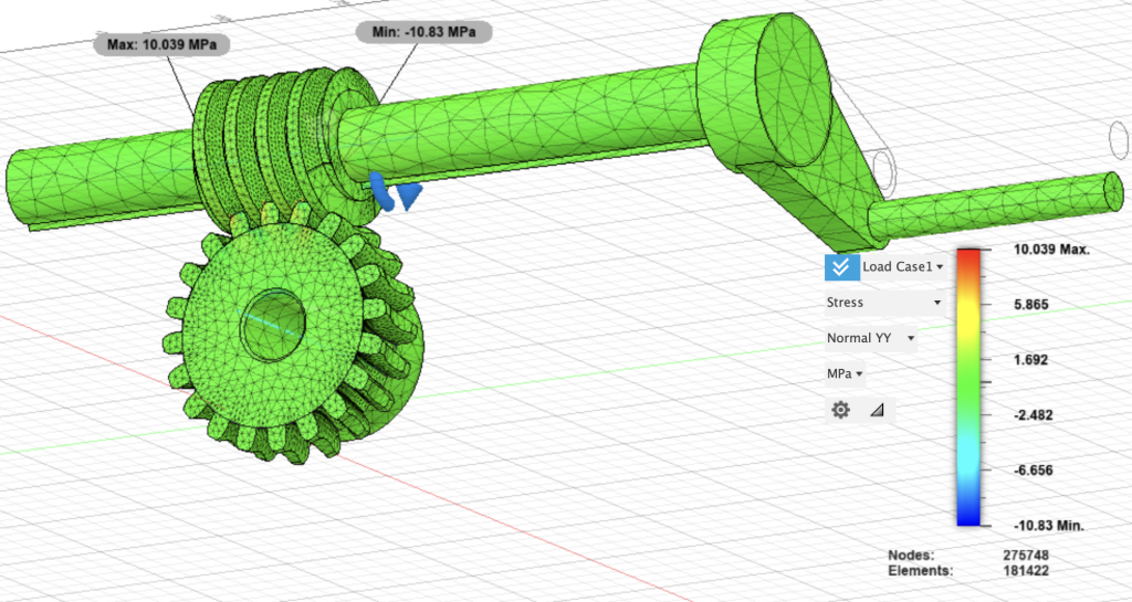
Figure 1 – Image of the constraints applied on the first true beam structure. The “Type” is “Fixed.” The Ux, Uy, and Uz degrees of freedom are selected next to “Axis.”

The loading cases offered extend beyond general distributed and point loads that most cantilever beam studies emphasized. For instance, there exists a “moment” load, which simulates an axial force being applied to a face or body; in this sense, the structure the load is applied to should rotate about a certain axis. Consider a shaft that turns a gear when rotated about the y (horizontal) axis. With the implementation of contact forces to simulate the force exchange between multiple connected structures, the following worm gear model was designed and the stress of the structure upon the moment load is barely visible.

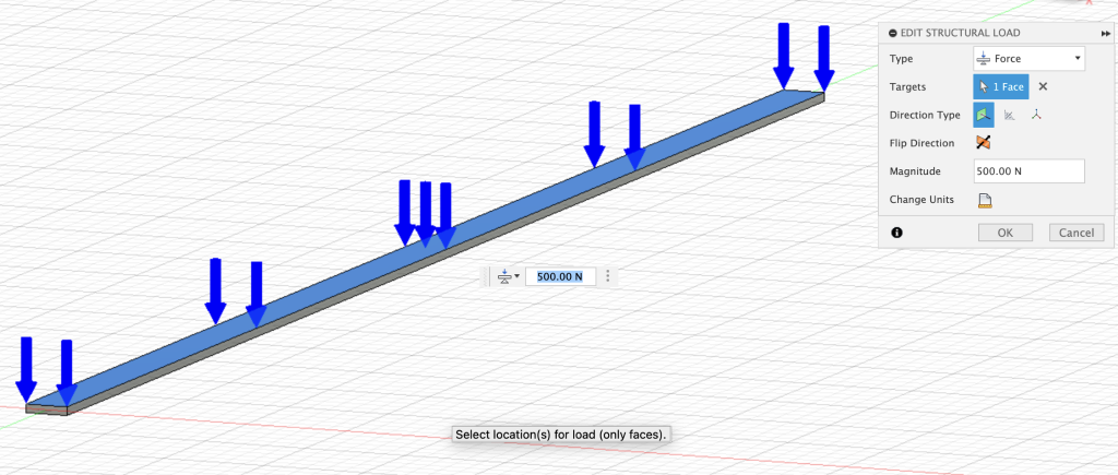
Figure 2 – Stress results of the worm gear structure with a moment load. Although not clearly visible, there are regions of red (high stress) at the intersection of the top and bottom gear.

For our specific cantilever beam problem, we consider the same stress factors that a moment load may cause, but impose a uniformly distributed load on the top face to deflect the beam in the Z direction. Granted that the variable we intend to predict is the linear deflection of a cantilever beam, it seems appropriate to utilize a load that can displace the beam vertically. We could also assign the load to the side faces at the ends of the beam, but we would receive a vibration along the Y axis with insignificant displacement values and the negative side effect of non-linear geometries. Additionally, the load remained constant at a magnitude of 500 Newtons across all variations of the beam geometry. See below:

Figure 3 – Image of a distributed load of 500 Newtons applied to the first true beam structure. While the force at the center has three arrows instead of two, the entire length of the beam experiences the same force.

The material properties included the finite element default for cantilever beams: steel design material with a young’s modulus of 210 GPa (2.1e+11 Pa), density of 7.850e-06 kg/mm³, and a poisson’s ratio of 0.30. For future reference, the most relevant feature among material parameters for the simulation model is the young’s modulus, as its value will be an essential component of the analytical calculations.

Finally, the mesh element sizes are characterized below:

Figure 4 – Image taken from the mesh settings popout in Fusion360. The main revision we made from the default Adaptive Mesh Refinement settings is reducing the Results Convergence Tolerance from 20% to 0.5% and multiplying the initial 10% of Portion of Elements to Refine by 4.

Figure 5 – Parameters for mesh refinement. While Fusion360 can automate a solid mesh for ease of use, we can refine the mesh further to increase the accuracy of the simulation’s results. A comparison between our custom mesh and Fusion’s standard mesh are expressed above.

Figure 6 – Summary of each mesh setting. This summary was produced from a beam mesh that we did not refine. However, it is important to consider from this summary that the mesh was split into 10 element solids—a feature that remained constant for all 72 beams.

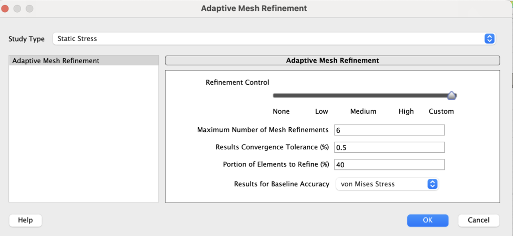
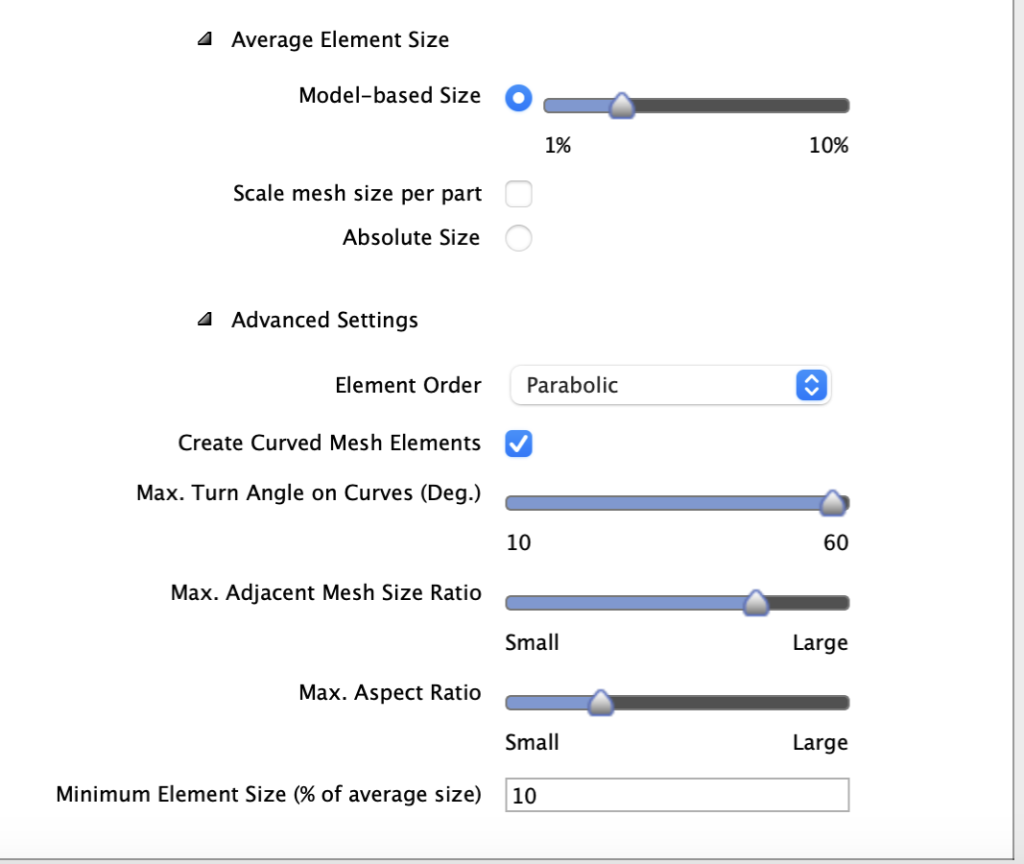
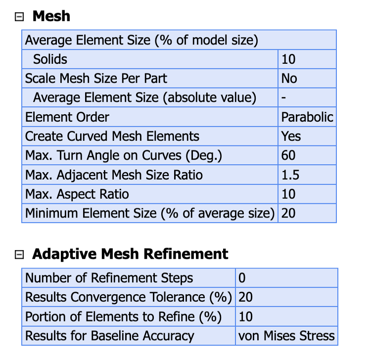
We followed other researchers who utilized finite element analysis for cantilever beams, implementing 10 solid elements. For about half of the true beam geometries, we refined the size of these elements to receive a smaller percent error between the exact deflections and the analytical solutions. The computational load for the adaptive mesh refinement is quite intensive, so we could not apply a finer mesh to each of the 36 beam cases.

We trained two different types of neural networks: a Feed Forward Neural Network coded in JavaScript and a Multi-Layer Perceptron coded in Python. Input data remains as the length, width, and height (in meters), while the output feature is deflection (in meters). The total data used to train the Multi-Layer Perceptron model is split with the following ratios:

	Number of Samples	Ratios (%)
Training	64	80
Testing	8	10
Validation	8	10

Figure 7 – Table explaining the counts of the training, testing, and validation set, and the relative ratio. The validation set comprise miscellaneous entries for length, width, height, and deflection unrelated to the actual dataset. This data ensures the model can perform accurately on unseen values.

For both types of networks, we built 1-layer, 2-layer, and 3-layer models with 10 nodes each. For the Feed Forward Neural Network, we plotted the loss of each model in MatLab, firmly concluding that the 3-layer model converged to a loss at or near zero in the least number of iterations/epochs.

Uniform Sampling of Data

In a dataset with uniformly arranged values of length, width, and height for a cantilever beam, the graph of the relationship between deflection and height should not vary to a high degree. Our dataset is ordered such that for every value of width that is constant, there are three distinct heights. The opposite also applies. The table below serves as a baseline for deriving the effect of uniform samples of data on deflection trends.

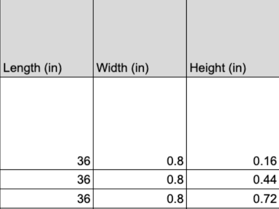
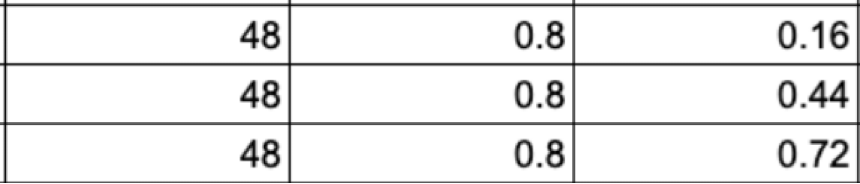
Figure 8 – Table displaying three beam structures with a length of 36 in where only the value of height increases by 0.28 in at each row and the width remains constant. (The dimensions are in inches to reduce significant figures and clearly display the trend).

Figure 9 – Table displaying a second iteration of three data points in which the beam length is 48 in, with the same increments of height as the previous set. Dimensions are still in inches and the column titles can be carried over.

The missing feature in these data subsets is the feature of interest: deflection. Each row of length, width, and height data is associated with both an exact deflection—the Z deflection calculated by the Fusion finite element simulation—and a “predicted” deflection—the δ calculated analytically. We will construct a two-dimensional graph with height values on the x-axis and FEM deflection values on the y-axis. The height data needed for the graph is listed above; in these cases, it is the only feature that can be considered an independent variable.

Figure 10 – Graph representing the Figure 7 3×3 data table with the addition of the corresponding deflection points.

Figure 11 – Graph representing the Figure 8 data table with the addition of the corresponding deflection points.

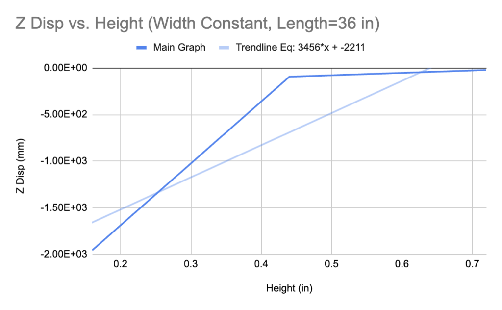
Despite the similar shapes of the graphs, there is a significant difference between their linearized slopes. It is clear that linearization is not the most optimal way to simplify this type of graph, but it can help us define implicit trends between deflection and beam dimensions. We can further quantify this relationship by plotting the data of the non-true beam deflections and heights in an identical fashion.

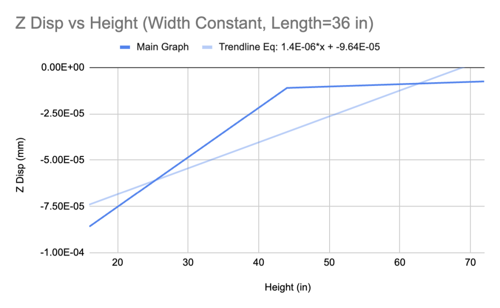
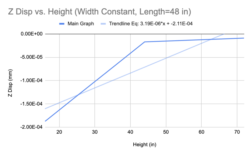
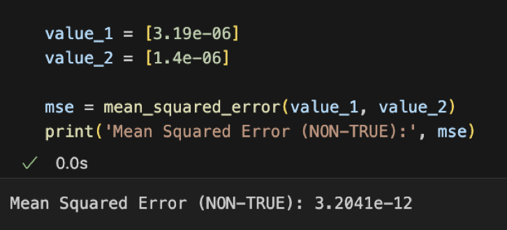
Figure 12 – Graph of the relationship between the beam’s displacement in the Z direction and the height of each beam, considering constant values such as width and length

Figure 13 – Graph of the relationship between the beam’s Z-displacement and the height of the beams, with the same conditions as the previous figure except for the change in length from 36 inches to 48 inches.

The similarity in the shapes of all four graphs suggests that it is reasonable for us to incorporate non-true beam geometries in the dataset. Further, the slopes of the trendlines for the non-true beam geometry cases return a substantially smaller mean squared error when compared with true beams. The metric can be skewed depending on the size of the number (smaller numbers always return lower mean squared errors), but still explains the distinction between two values more cohesively than simply taking the difference.

Figure 14 – Mean squared error between the slopes of the non beam specific linear graph from Visual Studio Code.

Figure 15 – Mean squared error between the slopes of the beam specific linear graph from Visual Studio Code.

Given that both geometries have underlying statistical similarities, the neural network training process will be considerably more comprehensive with the two datasets combined. This subtle addition has not yet been tested in the literature we described, but could contribute to reductions in loss during the prediction phase of our analysis.

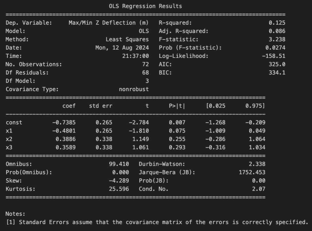
Additional observations were made from backend statistics modeling of feature inflation. OLS Regression StatsModels displays the independent effect of each input feature (i.e. length, width, and height) on the variance of the numerical output feature, deflection. Judging from the beta coefficient values in the “coef” column in Figure 16, length alone influences a 48% change in the value for deflection. Since the coefficient is negative, the relationship between length and deflection is an inverse one.

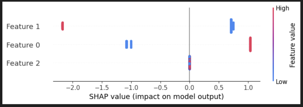
Figure 16 – Visual display of the Ordinary Least Squares (OLS) Statistics Model from the statsmodels API. To the left of the “coef” column, the “const” is the constant term added to the input data that standardizes values to prevent skews. The “x1,” “x2,” and “x3” are the features listed in the order we entered them in. The first feature is length, followed by width, and lastly height.

We can identify more discrete trends between the independent and dependent variables through Shapley Additive Explanations (SHAP). SHAP can derive the impact of a set of features on the output when trained to a regression model, accounting for the magnitude of the impact and the type of statistical relationship.

The regression model we selected was the Multi-Layer Perceptron (MLP) Regressor from sklearn’s neural network library. The solver for weight optimization is “lbfgs.” Additional parameters include an alpha of 0.001, maximum iterations of 400, and a maximum number of function calls at 200,000.

The following description refers to Figure 17 (below):

While length (m) may initially experience a negative relationship with the deflection data, we can discern that width (m) has a stronger inverse trend with the output after a more thorough analysis with the neural network. It is vital to note that the SHAP graph below took 5 minutes to render, indicating that this result is more dense than standard OLS regression statistics.

Figure 17 – Beeswarm SHAP plot measuring the positive and negative impact of each feature on the dependent variable (deflection). Negative impact values indicate a negative association between the feature and output variable, while positive impact values represent a positive association. Feature 0 is length (m), Feature 1 is width (m), and Feature 2 is height (m).

Discussion of The Analytical Formula

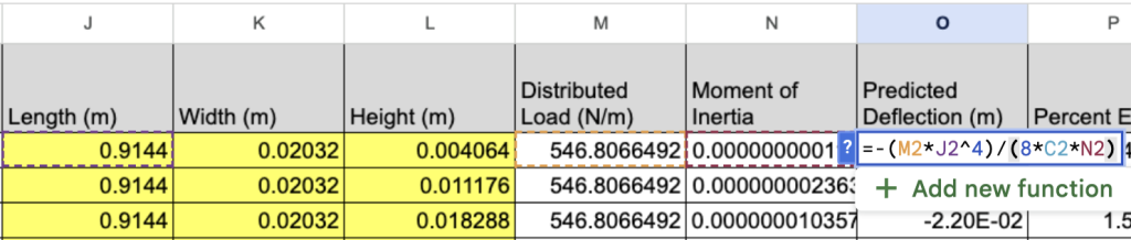
Figure 18 – A chart of the various different beam load cases and the deflection equations that independently refer to them. Based on boundary and loading conditions outlined in the methodology, analytical solutions were computed through the third equation. Standard units of meters are assumed for length (L), a shared variable in these equations. (https://www.omnicalculator.com/construction/beam-deflection)

The analytical equation for the deflection of a cantilever beam in a single case (eliminating the use of differentiation) varies based on the load case. Point loads displaced from the origin of the beam structure can make the analytical solution more difficult to compute. That is, more variables must be assigned data entries. In a uniform distributed load, the force is applied in equal proportions across the length of the beam. Accordingly, the value of the distributed load is the division of the 500 N force load we initialized by the length of the beam. This value is represented by the variable w in the equation below.

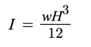
The alias of the young’s modulus is “E.” The product of the young’s modulus and the moment of inertia of the beam (I) is regarded as the bending stiffness. As implied by the equation, bending stiffness interacts with deflection in an inverse relationship: a greater stiffness would ensure a reduction in the deflection. With the data collected, we can define the moment of inertia with the following equation, where w is the distributed load and “H” is the height of the beam in meters:

The analytical solutions are listed under the “Predicted Deflection (m)” column of our dataset. These analytical deflections were calculated for non-true beam cases as well. To avoid the burden of performing 72 manual algebraic calculations without differentiation, we saved the function to the same Google Spreadsheet with our data.

Figure 19 – A cutout of our main dataset, emphasizing how the beam deflection equation has been imported into google spreadsheets. The predicted deflection contains a negative sign because the exact deflection in our finite element models occur in the negative Z (vertical) direction. The columns are assigned under letters ranging from J to N. For each row in the dataset, the saved function will substitute in the value in the column for the letter itself.

The percent error was found by comparing the predicted (analytical) deflections with the FEM (exact) deflections. Excluding non-beam cases, the minimum percent error we received was 0.12% and the maximum value was 6.2%. Because the analytical equation above is specific to cantilever beams only, the error for extraneous (non-true) geometries was 100% in all 36 cases. This error should not be confused with the mean squared error or loss returned by the neural network, since any deflections predicted by the model will be validated by the FEM deflections only.

Results of the Neural Network Model

Feed Forward Network (MATLAB)

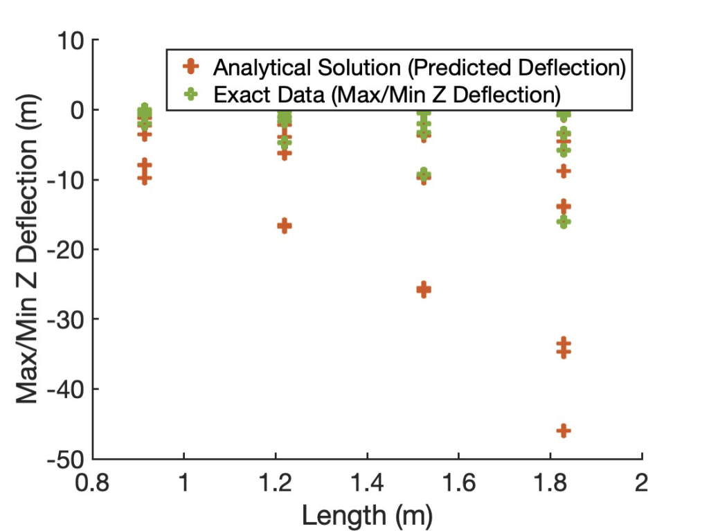
A feedforward neural network is a traditional deep learning network with less weights and node connections than other commonly-applied ones, such as the artificial neural network (ANN) explored by other researchers. This neural network was coded and calibrated in MATLAB, which allowed us to display the initial state of our data below. At this point, the analytical solutions of beam deflections represent our “predictions,” while the deflection values we recorded from the simulation form the exact data. Figure 20 (below) reveals the differences between the predicted and exact deflections across the length of each beam. Note that these differences can extend as far as 40 meters because we incorporated non-true beam geometries that do not follow the analytical equation provided in the previous section.

Pre-Training Difference between Exact and Analytical Solutions

Figure 20 – This graph displays the variation of the Z Deflection based solely on the length of the beam. In the legend, the predicted deflection (in red) refers to the analytical solution we calculated with the formula above. The exact data (in green) is the deflection we simulated with Fusion Computer Aided Design (C.A.D.).

For each 1-layer, 2-layer, and 3-layer neural network, we graphed the duration of epochs over which the network was trained on the input data (i.e. length, width, and height), as well as the resulting loss. Through each epoch, the neural network finishes one training iteration for all the input values. The network repeats this fitting process for 150 iterations. Ideally, the loss reaches zero before the 150th iteration. As such, the graph appears as that of an exponential function with a negative power (e.g.).

Figure 21 – Graph of Loss vs. Iteration for the Feed Forward Neural Network (ANN) with 1 Layer (10 Nodes)

Figure 22 – Graph of Loss vs. Iteration for the Feed Forward Neural Network (ANN) with 2 Layers (20 total nodes)

Figure 23 – Graph of Loss vs. Iteration for the Feed Forward Neural Network (ANN) with 3 Layers (30 total nodes)

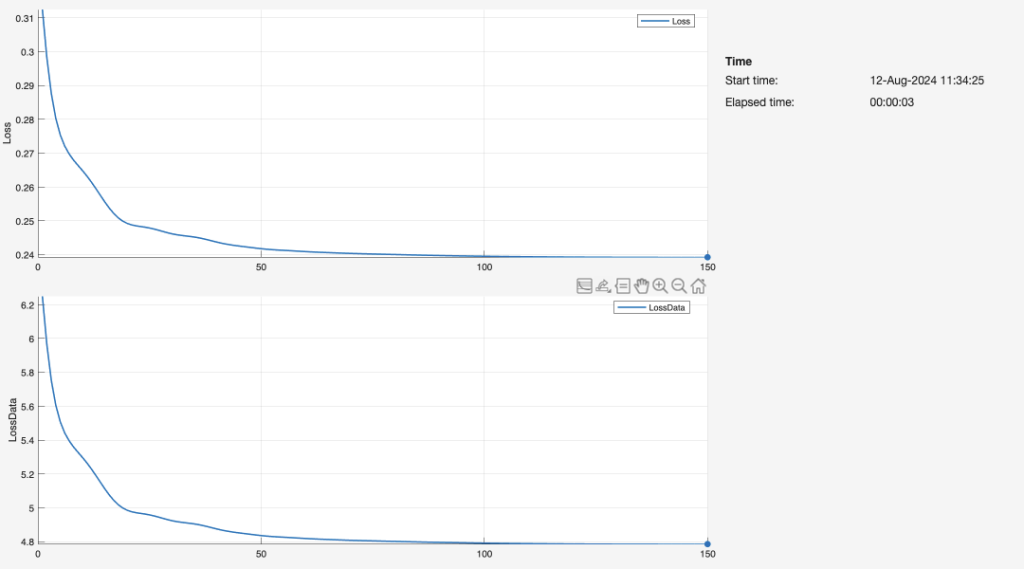
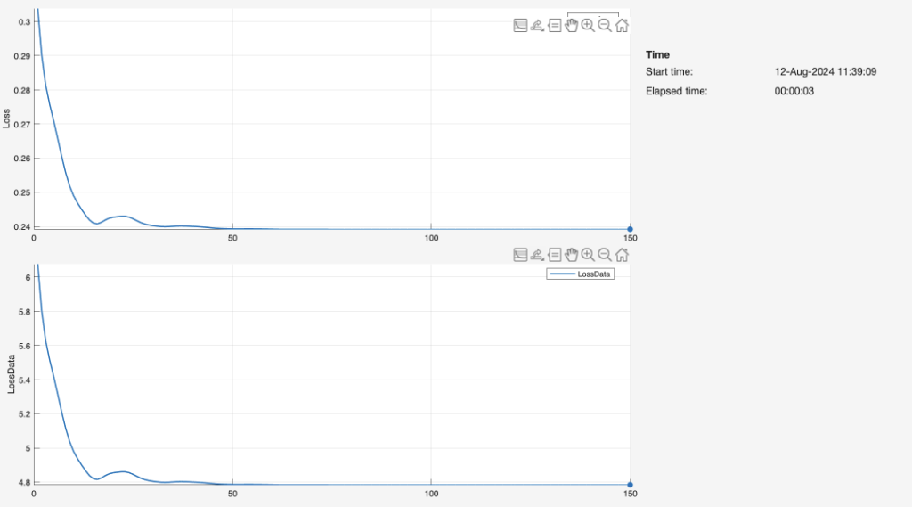
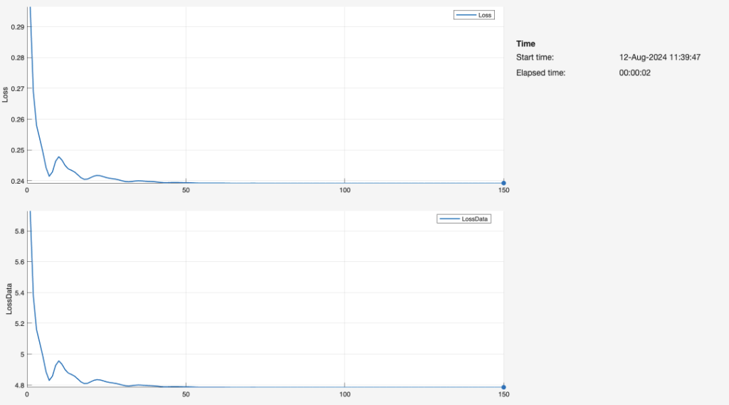
The number of layers is directly associated with the speed of the neural network. The three-layer network (Figure 23) delivers the fastest computation time, creating a reliable fit to the data by about 10-20 epochs. By comparison, the second-layer network is fairly similar in terms of the training process and resulting graph, but achieves a low loss at a greater number of iterations. The single-layer network is the least efficient by far, likely because it lacks a sufficient number of nodes and dense layers to interpret the data. Our observations in these plots of Loss vs. Iterations are greatly aligned with a Georgia Institute of Technology schematic (Figure 24):

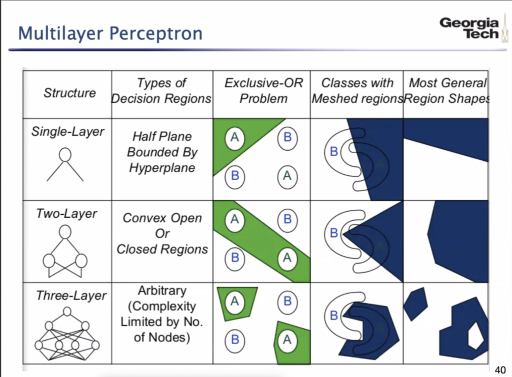
Figure 24 – Graphic from Georgia Institute of Technology describing how the neural network classifies the data into classes during the training process. (https://www.analytics.gatech.edu/curriculum/courses)

Considering that a three-layer neural network applies a more complex split to the meshed data, it can predict values closer to the those in the assigned testing or validation set. A simpler shape or class would increase the likelihood of error, as there is increasing overlap in the regression ranges that the model dictates in order to classify and ultimately predict deflection.

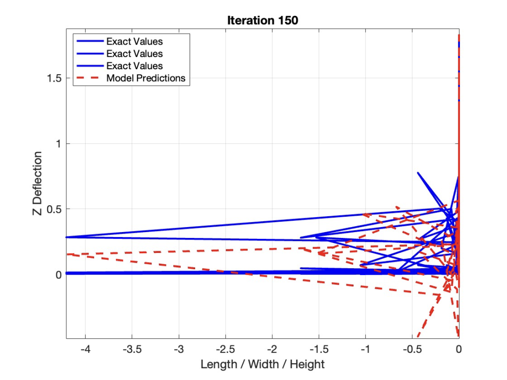
Figure 25 – The training progress graph (Loss vs. Iterations) for a three-layer feedforward network that corresponds with Figure 26 below.

Now that the training process is complete for the feedforward network, we tested the performance of the 3-layer model by displaying the difference between its predictions and the exact FEM simulation deflections. A line chart (Figure 26) reveals the accuracy of the predictions after 150 iterations, assuming the training loss reaches zero after less than 50 iterations.

Figure 26 – A line chart that shows the convergence of actual and predicted values at 150 iterations. Lines are color-coded such that blue solid lines represent the exact data produced by the Fusion simulation, and red dashed lines correspond to the predicted values computed through neural network. (“Exact values” is repeated three times in the legend, because the neural network can fully process a batch of input data with zero loss after 50 iterations).

Results from the Validation Trial

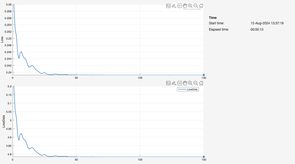
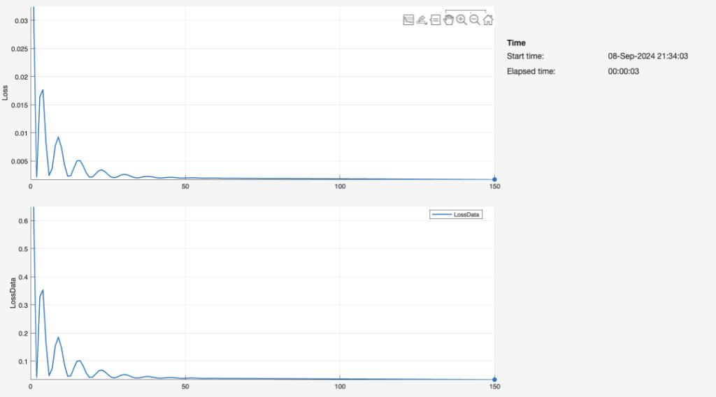
We tabulated the deflection values that the model predicted from a random validation set of length, width, and height data. The inputs as such were populated randomly by us. Then, we designed eight additional structures based on these dimensions. Similar to our original procedure for the first 72 beam variations, we ran a “Static Stress” simulation on each structure through Fusion360. The simulated deflections are listed as “Max/Min Z Deflection (m).” Our feedforward neural network was first trained on the beam dimension values. Figure 27 describes the values of loss graphed over the number of epochs for the training process. The loss likely fluctuates because the input values are entirely arbitrary; they do not follow a uniform trend of any kind. After predicting deflection in the same fashion as our main experiment and methodology, we recorded the predictions and pasted them to the right of the deflected values produced by the simulation. Figure 28 and Figure 29 (below) quantify the difference between the true and predicted deflections, extending the graphic of Figure 26.

Figure 27 – Graph of loss vs. iterations for the 3-layer feedforward neural network when trained on the length, width, and height data from the validation set.

Length (m)	Width (m)	Height (m)	Max/Min Z Deflection (m)	Feed Forward Predicted Deflections (m)
1	0.075	0.03	-0.002	-0.0979
1.75	0.03	0.01	-0.623	-0.2684
1.1	0.06	0.006	-0.353	-0.1454
1.3	0.07	0.015	-0.031	-0.1628
1.6	0.04	0.025	-0.023	-0.2241
0.95	0.025	0.008	-0.235	-0.1445
1.4	0.045	0.015	-0.062	-0.1968
1.9	0.08	0.012	-0.172	-0.2552

Figure 28 – Data table reflecting the validation set’s independent variables (Length, Width, Height) and dependent variables (Max/Min Z Deflection), with the addition of the deflection values predicted by the feedforward network. For ease of comparison, the predicted and exact values of deflection are side by side.

Figure 29 – Mean squared error between the feedforward network predictions and the simulated values of deflection (taken directly from the Figure 28 table above) from Visual Studio Code

Multi-Layer Perceptron (Visual Studio Code)

Feedforward neural networks are a raw deep learning network of logistic regression systems, where not every layer is fully connected. With MATLAB’s feedforward networks, we can visualize the training process, loss, and difference between the predicted and actual deflection values in a graphical form. Further, a multi-layer perceptron (MLP) network is a more developed version of the feedforward neural network; each node in an MLP has a connection to every other node in the subsequent layer. We trained this additional network on our data to assess whether the accuracy of our current deflection predictions can improve.

In order to maximize the efficacy of the multi-layer perceptron network, we had to refine its parameters, including the activation function, the optimizer, and the number of iterations (epochs) that the network would pass through the training samples. Initially, the loss of the MLP network was inconsistent, returning extremely high losses in some runs and significantly low losses in others. After several trials, we concluded that the Rectified Linear Unit, or “ReLU,” activation function caused this fluctuation in loss. When substituting this method with the Softplus activation function—a more non-linear, smoother replica of ReLU—the loss declined. Specifically, with a Softplus activation, the mean squared error falls to a steady range of 0.05 to 0.08.

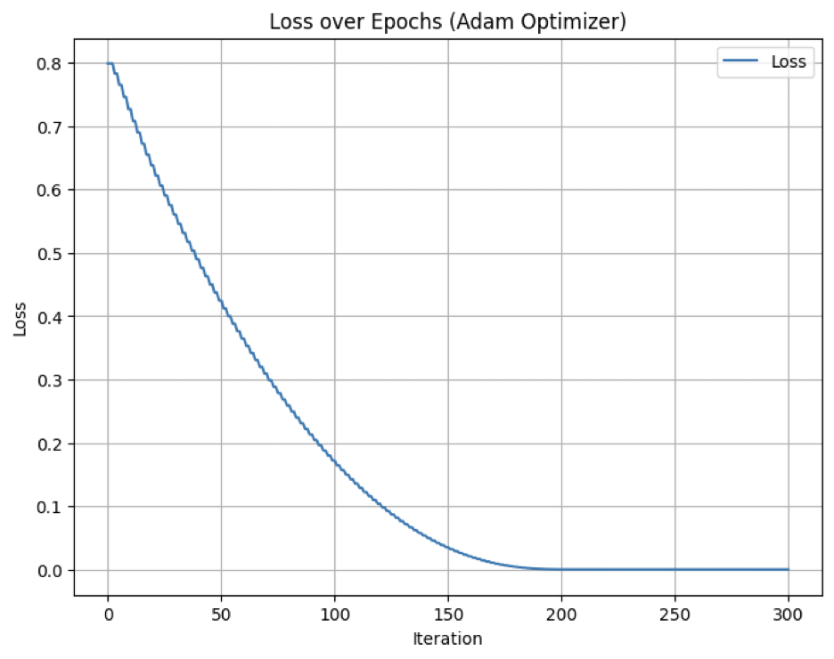
Each neural network requires an optimizer as an internal parameter that can streamline the process of assigning weights and learning from the data. As such, optimizers contain hyperparameters such as learning rates, where high learning rates cause the neural network to converge to a solution faster. We graphed the loss of the Adam optimizer with a learning rate of 0.01 and recorded the number of epochs the model would take to fit the data such that the loss of optimizer reaches zero. Results varied within the range of 150 to 300 epochs. The most consistent result, however, was a loss convergence of 0 beginning at 175 epochs and and ending at 300 epochs. Accordingly, if our multi-layer perceptron takes between 175 and 300 epochs to train the data, we will avoid stopping the model before the optimizer of the network attains its minimum loss. Thus, the loss of the network as a whole should decrease to a number closer to 0. We incorporated an additional “Early Stopping” method to verify that the model’s loss continuously decreases across each epoch. That is, if no improvement in loss is observed after 5 or 10 epochs, the network instantaneously stops running.

Figure 30 – The graph of Loss vs. Iteration (epochs) for the Adam optimizer. It follows the same decreasing trend as the loss graphs of the feedforward network.

Granted that the Adam optimizer is generally observed in large datasets, it was crucial to define the “gradient_accumulation_step” hyperparameter associated with this optimizer in this case. For context, we collected only 72 rows of data with four corresponding columns, making our data decisively small. In a practical sense, a smaller gradient step ensures that gradients—measurements of the difference between weights assigned to each node and the resulting loss—are applied less frequently. For our multi-layer perceptron network, a decrease in the gradient accumulation step from a value of 5 to 2 had substantially reduced our total network error.

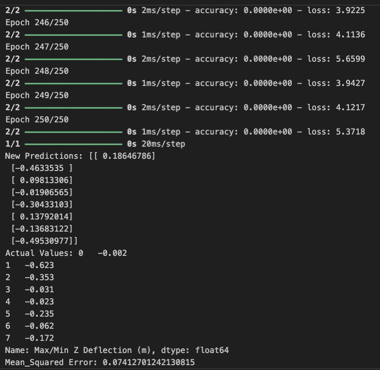
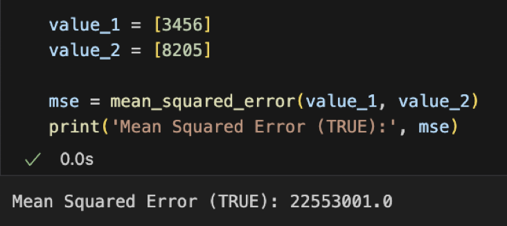
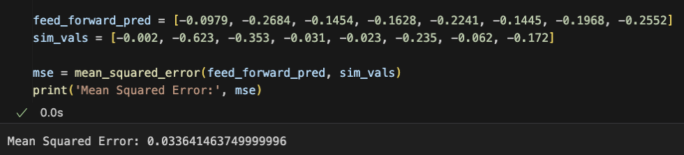
Figure 31 – The post-training results of the MLP model are displayed above. Predicted values for deflection were returned for a random set of beam dimensions that conformed to true beam geometries; they are listed as “New Predictions.” The simulated results for the same set of dimensions were stored in the list, “Actual Values.”

When fitting the neural network with the most optimal hyperparameters, we reach a loss of zero. We forced the model to predict the values of deflection based on a random training set of cantilever beam geometries, and recorded the mean squared error between the predicted values and the corresponding testing values. As we hypothesized in our discussion about the Adam optimizer, the margin of error is almost insignificant. Considering that the model was tasked with predicting values based on unseen data, the results are impressive, regardless of the ~0.2 m difference between the “New Predictions” and “Actual Values” listed above.

Overall, when tested on a validation set of random values, the feedforward neural network can predict deflection with more than twice as less error as the multi-layer perceptron. In other words, the mean squared error of the MATLAB feedforward neural network was approximately 0.034, while that of the multi-layer perceptron built in VS Code was 0.074. Unlike a standard feedforward neural network, a multi-layer perceptron network is unique in that each node in the hidden layer of an MLP connects to every other node in the next layer. It is possible that the feedforward network is more accurate due to the simplicity of our dataset; that said, more research surrounding the association between this network and the size of datasets is still needed. Because the common issue of overfitting is a direct result of the model performing poor on testing data it has not been fitted to, we instructed the model to predict eight rows of deflection data from distinctly random input values for length, width, and height. We discovered that overfitting was not a direct cause of inconsistent or abnormally high losses in the network fitting process, but rather the error could be attributed to the inefficiency of our optimizer and activation function.

Conclusion

Beam deflection is computationally expensive to predict through Finite Element Analysis, but we have proven that this inefficiency can be reduced through training a feedforward and MLP neural network on the same beam data. Designing a beam structure with specific dimensions and simulating its deflection may take upwards of an hour to produce results accurate to the 0.1%, depending on the size of the mesh. Alternatively with deep learning models, we can receive the values for beam deflections in less than thirty seconds in most cases. The finite element method is limited by the physical shape and properties of a structure, raising implications for the implementation of similar neural networks in future physics-related projects. For cantilever beams specifically, it would be especially pertinent for engineers to refer to an application where they can instantly find the deflection of a steel beam by entering the length of the beam and the type of load (refer back to Figure 20). While such tools may already exist, given that the analytical solution for cantilever beam deflection is widely known, there are massive opportunities in the field of non-linear beam geometries, where deflection varies in a pattern that cannot be defined analytically or with FEM simulation parameters that are not updated regularly.

Deep learning offers an expanse of opportunities for optimizing modern buildings and structures. Since the invention of the first flying object, airplane wings have experienced little relative change in terms of improving aerodynamic efficiency. Aeronautical engineers play a crucial role in innovating new airfoil designs for maximizing lift, for example, but we will eventually reach a point where generative artificial intelligence outpaces Computer Aided Design (C.A.D.) and finite element simulations, both of which are quite dated. Physics-Informed Neural Networks (PINNs) are becoming increasingly popular in the landscape of artificial intelligence, as they can interpret differential equations and existing data to predict complex physics trends. In fact, these newfound neural networks can approximate analytical physics solutions with little data, if any at all; even the state-of-the-art machine learning models fail in that context. Ultimately, with the increasing complexity of engineering projects today, C.A.D. simulations are inherently more prone to error. Through this project, we predicted a physics trend applied frequently in structural engineering cases to a degree not only as accurate as the most dense FEM simulations, but also more sustainable.

Figure 32 – The Fusion360 C.A.D. model of a sample airfoil from Airfoil Tools. It is highlighted for its three meshing errors that occur at various regions of the model. This attempt at establishing a static stress simulation for a plane wing reveals how intensive the solving process can be for complex structures. In this sense, there are too many variables to account for.

Citations

Chaphalkar, S. P., et al. “Modal analysis of cantilever beam Structure Using Finite Element analysis and Experimental Analysis.” American Journal of Engineering Research (AJER), vol. 4, no. 10, 2015, pp. 178-85, www.academia.edu/27362678/
Modal_analysis_of_cantilever_beam_Structure_Using_Finite_Element_analysis_and_Experimental_Analysis. Accessed 9 Sept. 2024.

Kimiaeifar, A., et al. “Large Deflection Analysis of Cantilever Beam under End Point and Distributed Loads.” Journal of the Chinese Institute of Engineers, vol. 37, no. 4, Aug. 2013, pp. 438-45, https://doi.org/10.1080/02533839.2013.814991. Accessed 9 Sept. 2024.

Kocatürk, T., et al. “LARGE DEFLECTION STATIC ANALYSIS OF A CANTILEVER BEAM SUBJECTED TO A POINT LOAD.” International Journal of Engineering and Applied Sciences, vol. 2, no. 4, 2010, pp. 1-13, dergipark.org.tr/tr/download/article-file/217635. Accessed 9 Sept. 2024.

Lam Thanh Quang, Khai, et al. “Structural Analysis of Continuous Beam Using Fem and Ansys.” JOURNAL of MATERIALS & CONSTRUCTION, vol. 11, no. 02, 17 Mar. 2022, https://doi.org/10.54772/jomc.v11i02.291. Accessed 9 Sept. 2024.

Mekalke, G. C., and A. V. Sutar. “Modal Analysis of Cantilever Beam for Various Cases and its Analytical and Fea Analysis.” International Journal of Engineering Technology, Management and Applied Sciences, vol. 4, no. 2, Feb. 2016, pp. 60-66, www.researchgate.net/publication/318760743_Modal_Analysis_of_Cantilever_Beam_for_Various_Cases_and_its_Analytical_and_Fea_Analysis.

Oladejo, Kolawole Adesola, et al. “Model for Deflection Analysis in Cantilever Beam.” European Journal of Engineering Research and Science, vol. 3, no. 12, 18 Dec. 2018, pp. 60-66, https://doi.org/10.24018/ejers.2018.3.12.1004. Accessed 9 Sept. 2024.

Samal, Ashis Kumar, and T. Eswara Rao. “Analysis of Stress and Deflection of Cantilever Beam and its Validation Using ANSYS.” Ashis Kumar Samal Int. Journal of Engineering Research and Applications, vol. 6, no. 1, Jan. 2016, pp. 119-26, ijera.com/papers/Vol6_issue1/Part%20-%204/Q6104119126.pdf. Accessed 9 Sept. 2024.

Sargent, Brandon S., et al. “The Mixed-Body Model: A Method for Predicting Large Deflections in Stepped Cantilever Beams.” Journal of Mechanisms and Robotics, vol. 14, no. 4, 18 Feb. 2022, https://doi.org/10.1115/1.4053376. Accessed 9 Sept. 2024.

Tuan Ya, T.m.y.s, et al. “Analysis of Cantilever Beam Deflection under Uniformly Distributed Load Using Artificial Neural Networks.” MATEC Web of Conferences, vol. 255, 2019, p. 06004, https://doi.org/10.1051/matecconf/201925506004. Accessed 9 Sept. 2024.

Wang, Tianyu, et al. “A Deep Learning Based Approach for Response Prediction of Beam-like Structures.” Structural Durability & Health Monitoring, vol. 14, no. 4, 2020, pp. 315-38, https://doi.org/10.32604/sdhm.2020.011083. Accessed 9 Sept. 2024.

Brownlee, Jason (January 24, 2019), “Understand The Impact Of Learning Rate On Neural Network Performance”, Machine Learning Mastery, Guiding Tech Media https://machinelearningmastery.com/understand-the-dynamics-of-learning-rate-on-deep-learning-neural-networks/. Accessed on September 9, 2024.

Airfoil Tools (January 1, 2024), “Airfoil Tools”, http://www.airfoiltools.com/. Accessed on September 9, 2024.

ALEX (April 8, 2020), “Feedforward Neural Networks And Multilayer Perceptrons – Boostedml”, Boostedml, All Right Reserved, https://boostedml.com/2020/04/feedforward-neural-networks-and-multilayer-perceptrons.html. Accessed on September 9, 2024.

Papers With Code (September 30, 2017), “Softplus Explained | Papers With Code”, Papers With Code, https://paperswithcode.com/method/softplus. Accessed on September 9, 2024.

Alambra, Kenneth (November 28, 2018), “Beam Deflection Calculator”, Omni Calculator, , https://www.omnicalculator.com/construction/beam-deflection. Accessed on September 10, 2024.

Tech, Georgia (January 1, 2024), “Courses | Master of Science in Analytics”, Master of Science in Analytics, Georgia Institute of Technology, https://www.analytics.gatech.edu/curriculum/courses. Accessed on September 10, 2024.