Quantum Approximate Optimization Algorithm for the Max-Cut Problem: Performance Comparison with Classical Approaches on NISQ Devices

Abstract

The Max-Cut problem is a foundational NP-hard combinatorial optimization problem with quite a few uses, such as circuit and semiconductor design, financial modeling, and data flow optimization. The exponential nature of the problem makes scalability over large inputs infeasible, making it a benchmark for solving such problems using methods like quantum computing due to them being infeasible for classical algorithms in such situations.

While the Quantum Approximate Optimization Algorithm (QAOA) has shown theoretical promise for solving such problems, the practical threshold at which quantum approaches outperform classical methods on real noisy intermediate-scale quantum (NISQ) devices remains unclear. This paper aims to resolve this uncertainty. The investigation itself compares the performance of QAOA executed on IBM’s 133-qubit Torino quantum processor for the Max-Cut problem on modern quantum devices and compares its performance against the classical brute-force method in order to gauge the potential advantage that quantum algorithms may provide as input size grows. It consists of running both algorithms over (unweighted) graph sizes ranging from 4 – 24 nodes for 5 independent trials each, measuring both execution time and approximation ratio. The QAOA implementation uses a circuit with a singular fixed depth and fixed Hamiltonian parameters to ensure consistency over all trials & fairness in comparisons between graph sizes. However, this along with noise leads to a low chance of the optimal cut being produced.

The classical solver exhaustively evaluated all 2ⁿ possible partitions to produce the optimal cut value. Classical execution time grew exponentially from 0.16 milliseconds (4 nodes) to 87.6 seconds (24 nodes), consistent with the brute-force algorithm’s behavior. On the other hand, QAOA maintained near-constant execution time (~1.33 seconds across all graph sizes), with both approaches converging at approximately 19 nodes. However, QAOA’s approximation ratio declined from 0.95 (4 nodes) to 0.52 (24 nodes), reflecting limitations of shallow circuit depth and hardware noise. These findings demonstrate that QAOA exhibits superior scalability as graph size increases compared to exact classical methods but due to the limitations of NISQ quantum hardware, is unable to achieve this for large graph sizes, where it can be most practical, without accuracy as a trade-off. As quantum hardware advances in the future, high circuit depth will be possible with low noise or even error correction, which is expected to strengthen the performance of algorithms like QAOA substantially, allowing its theoretical advantages to be reaped to the fullest at solving NP-hard problems like the Max-Cut.

Key words:  compare, evaluate, execution time, approximation accuracy, scalability

Introduction

Optimization

In mathematics and computer science, optimization is a process that involves finding the best solution from the search space according to some defined criteria, while following certain rules/constraints according to the problem situation (Wright, 2025). 

The search space, in the context of optimization, refers to the set of all possible solutions that adhere to the problem’s constraints or objectives. Thus, it represents the feasible solutions that can be evaluated to find the optimal solution according to the objective function (Wright, 2025), which is a mathematical expression that defines the goal of an optimization problem, which is usually to maximize or minimize a quantity. It quantifies the desired outcome, serving as a guide for decision making and showing how close a solution is to the desired one (Fiveable, n.d.).

Combinatorial Optimization

Combinatorial optimization is a type of discrete optimization that refers to problems on discrete structures such as graphs. It aims to find the best or optimal solution to problems that have a finite set of possible solutions (discrete search space), and the best solution is usually the one that minimizes or maximizes the problem’s objective function (Lee, 2010; DeepAI, n.d.).

For each combinatorial optimization problem, there is a decision problem, which, in simple terms, is a yes/no version of it. It asks whether there is a feasible solution to the problem using a measurement threshold (Jaillet, 2010). For instance, given 10 interconnected cities, the optimization problem would be to find the shortest path from city a to city b. A corresponding decision problem would be to determine whether or not there is a path from city a to city b that crosses less than or equal to 5 intermediate cities.

Due to the nature of decision problems, if one can come up with an answer to it, that means the corresponding optimization problem is ‘feasible’ – a solution exists that satisfies all the constraints of the problem. Failing to do so means that the corresponding optimization problem is ‘infeasible’, or that no solutions exist that satisfy all constraints of the problem. Even if a problem is feasible, it may not necessarily be ‘bounded’, that is, there is no limit to how “good” or “optimal” the solution can get for the objective function. Thus, if an optimization problem is not infeasible and not unbounded, it must have an optimal solution and is therefore solvable (Maltby & Ross, n.d.).

The Max-Cut Problem

Now that discrete optimization and combinatorial optimization has been made clear, it is now appropriate to visit the ‘Max-Cut Problem’, a famous example of combinatorial optimization and the focus of this paper.

Let there be a graph G = (V,E)   with vertices V  and edges E . For starters, a graph in this context refers to a set of vertices/nodes in a 2-D space, which are mathematical abstractions corresponding to objects associated with each other by some criteria in place and are connected to one-another in some form by a set of edges E , each of which connects 2 nodes (Luca, 2023). Let there be a partition that divides set   V into 2 disjointed sets of vertices  A and  B. An edge is said to be “cut” by the partition if it connects 2 vertices that are not in the same set. Thus, the objective of the Max-Cut problem is to find a partition of vertices  V into complementary subsets A  and  B in graph V  that maximizes the edges between them (Goemans & Williamson, 1995). An example is shown in the figure below.

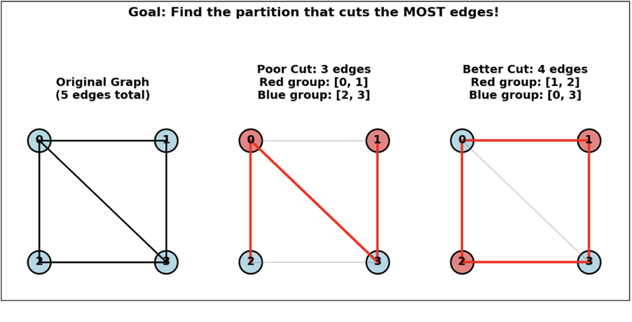
In the figure above, the image on the left shows the original graph with its set of nodes and edges. The image in the center shows nodes 0 and 1 in the red set and nodes 2 and 3 in the blue set, and it shows the possible cuts with that node with that specific set distribution (not the maximum cut), which is 3 cuts. The image on the right, however, shows the set distribution that gives the maximum number of cuts for the graph, which is 4 cuts – nodes 1 and 2 in the red set and nodes 0 and 3 in the blue set. It is important to note that distributing all nodes in the opposite sets – nodes 0 and 3 in the red set and nodes 1 and 2 in the blue set – will also give the same result because the edges that are “cut” will still connect nodes in different sets, which is all that matters. Note that any explorations of the Max-Cut problem in this paper deals with unweighted graphs, and the concept of weightage is being ignored entirely.

When checking whether the Max-Cut problem is solvable for all input sizes, firstly, it is imperative to assess its feasibility. To do so, assess the decision version of it, which is the following: Given a graph k   and an integer k, determine whether there is a cut value of at least   (Goemans & Williamson, 1995). It is indeed possible to have a cut of some value. Take the example in Fig.1 for instance. Let k be equal to 3; on the graph in the middle, a cut value of at least 3 is indeed possible. Thus, as the decision version is solvable, the max-cut problem is feasible. Lastly, it is imperative to assess its boundedness. As the name suggests, the Max-Cut problem must have a maximum possible cut value for a specific graph. To prove this, take the example in Fig.1 once more. The graph on the right side of the figure shows the maximum possible cut value for the given graph. If two nodes of the same set are adjacent to one-another, the maximum possible cut value is 3, which is shown by the graph in the middle, but if they are opposite each other, which is shown by the graph on the right, each node in the rectangular portion of the graph (and not the diagonal – the edge between node 0 and node 3) is connected to a node of the opposite set, maximizing the cut value for the given graph, which is 4. As there is a maximum cut value for this graph, specifically, there has to be a maximum cut value for every other graph with any number of vertices and combination of edges. This shows that the Max-Cut problem is bounded. Therefore, as it is both feasible and bounded, it is solvable.

        Although the objective of the Max-Cut problem may seem straightforward, no solution has been developed that can find the optimal solution in an efficient manner in all cases due to the nature of the statement problem, the limits of modern hardware, and scalability issues. Due to this, various approximation algorithms have been created to deliver suboptimal solutions, and quite a few of them utilize principles of quantum mechanics to do so, which allow parallel computations, that is, the ability to evaluate multiple possibilities at once. This is because the addition of a single qubit gives rise to exponentially more states and possibilities, giving quantum computers the ability to solve problems exponentially faster than classical algorithms (Tepanyan, 2025). A few classical approximation algorithms that have had sufficient success in approximating the Max-Cut problem are those using ‘greedy algorithms’ (Codecademy, 2022) and the ‘Goemans-Williamson Algorithm’ (Toni, 2018). However, these are not as effective as quantum algorithms, such as those using the ‘Quantum Approximate Optimization Algorithm’ (QAOA) (Ceroni, 2025) and Quantum Genetic Algorithms (QGA) (Viana & Neto, 2024).

As mentioned in the previous paragraph, both classical and quantum approximation algorithms have made progress in addressing the Max-Cut problem, but their effectiveness in practice depends heavily on the underlying hardware and the scalability of the method used. This raises an important question: when do quantum algorithms outperform their classical counterparts? Addressing this question motivates the main objectives of this paper. Specifically, we aim to explore and demonstrate the feasibility of running QAOA for the Max-Cut problem on real quantum devices and to compare its performance against the classical brute-force method (AlgoEducation, n.d.) in order to gauge the potential advantage that quantum algorithms may provide as input size grows.

Our work is driven by the hypothesis that while classical algorithms excel at solving problems with small to medium-sized input values at a great degree of efficiency, they become infeasible for solving large problems, and that quantum approaches, such as QAOA, have the potential to surpass them as the input size increases

Background – Classical vs. Quantum Approaches

Computational Complexity

To understand why quantum solutions are usually superior to classical solutions, it is imperative to understand why classical solutions can fail, for which the knowledge of computational complexity is needed. Computational complexity is a measure of how difficult a computational problem is and how much time is required to solve it. The Max-Cut problem specifically, is an ‘NP-Hard’ problem.

For an ‘NP’ hard problem, a proposed solution can be verified in polynomial time, but the solution itself cannot be found as quickly. Examples of NP problems are the ‘Boolean Satisfiability Problem’ (SAT) and the Sudoku Puzzle (Kanwal, 2021).

A problem is ‘NP-Hard’ if every problem in NP can be reduced to it in polynomial time, that is, if an NP-Hard problem can be solved efficiently (in polynomial time), all NP problems can be solved efficiently (Kanwal, 2021). In fact, quite a few NP-Hard problems are not even in NP because their solutions cannot be verified in polynomial time.

The reason why the Max-Cut problem, or the optimization version at least, is NP-Hard is because of two reasons. Firstly, it is indeed possible to count the edges cut, but it is not possible in all cases to verify that a certain partition of the vertices in set V  gives the maximum cut without essentially solving the problem itself. Secondly, it is a fact that as the number of vertices increases linearly, the number of possible partitions increases exponentially, which is why no perfect solution in polynomial time can exist for the Max-Cut problem.

Classical Solutions to the Max-Cut Problem

The max-cut problem can be written as a quadratic optimization function. To know why classical methods are not ideal, it is necessary to understand the structure of this objective function (Lowe, 2025), which reveals the very nature of the Max-Cut problem. Let  G = (V,E) be a graph with vertices   V and edges E  , and let  w_ij​ denote the weight of edge (i,j)  . This paper utilizes unweighted graphs, so w_ij = 1   . The variables x_i E { -1,1}   are binary variables for each vertex, representing the set assignment of the vertex – which subset of the partition it belongs to – that is A or B. The objective function can then be expressed as:

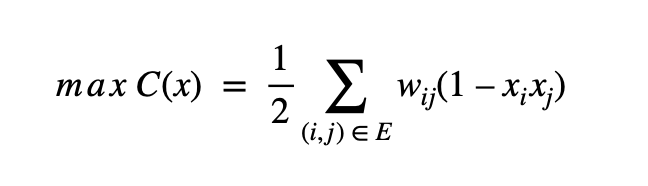
For each edge (i,j)  connecting vertices x_i  and x_j  , if vertices x_i  and x_j  are in the same subset, their product will be equal to 1, and since 1 – 1 = 0, the edge connecting x_i  and x_j  is not cut and it will not contribute to the cut value of  G. If x_i  and x_j  are in two different subsets, their product will be equal to -1, and since 1 – -1 = 2, the edge connecting x_i  and x_j  is cut and it will contribute to the cut value of  G (Lowe, 2025). Each existing vertex combination (x_i , x_j) in G is considered twice: once for (x_i , x_j)  and the other for (x_j , x_i)  because technically, they are not exactly the same vertex combination. However, in actuality, they connect the same edge, so to avoid such double counting, the total cut value after iterating after summing through every valid vertex combination is divided by 2. Therefore,  C(x) calculates the total cut value of graph G  , which is the same as calculating the maximum possible cut value for G  , which fulfills the objective of the Max-Cut problem.

Each vertex can be in one of two possible subsets. Because of this, the solution space of graph G  , or total number of possible partitions is 2ⁿ , where n  represents the number of vertices in G . Therefore, as the value of n  increases, the number of possible partitions increases exponentially, which starts to become infeasible after a certain point, especially for large values of  , because the time and resources required to iterate over all 2ⁿ   possible combinations become too large. This is why the function encoded by C(x) is NP-hard, due to which almost all algorithms created to attempt a solution at the Max-Cut problem are approximation algorithms. These are designed to produce near-optimal solutions within reasonable time limits, rather than iterating over all 2ⁿ  possible partitions, which is known as the brute force method – theoretically the only algorithm with an approximation ratio of 1.

One of the simplest classical approximation approaches is using a greedy algorithm (Codecademy, 2022), which is a technique that assigns vertices to the set that yields the largest ‘immediate’ increase in the cut size. Due to this aspect, despite their speed, greedy approaches often get stuck in locally optimal configurations that are not globally optimal. A significantly more powerful classical approach is the Goemans–Williamson algorithm (Cai, 2003), which uses a mathematical technique called semidefinite programming (SDP) to represent vertices as unit vectors on a hypersphere followed by randomized rounding to generate a cut. This is the most powerful classical approximation algorithm and is guaranteed to achieve an approximation ratio of at least 0.878, that is, to produce a cut that is guaranteed to be at least 87.8% as good as the optimal cut value, regardless of graph size.

Although such classical approximation algorithms are considerably efficient, their performance starts to diminish for very large or dense graphs, motivating research on alternative methods – quantum methods.

Introduction to Quantum Computing – For the Max-Cut Problem

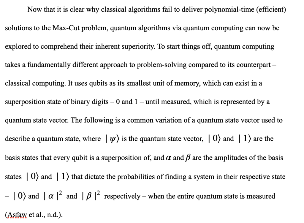
When multiple qubits are combined, they can represent an exponentially large number of possible states at the same time. This means that for a system with   qubits, its state can be described by a complex state vector in a 2ⁿ -dimensional space. This property of superposition (Thomson, 2025) of a quantum state is extremely valuable as it enables it to represent all 2ⁿ  basis states. Such simultaneous representation makes quantum parallelism – the ability of a single operation (in this case, a unitary operation) to act on all superimposed states at the same time – possible (Kaye & Mosca, 2020), which is the very thing that gives quantum computing the edge over classical computing: While a classical computer must check all 2ⁿ  possible combinations one at a time, a quantum computer can describe them all as a superposition of states representing those combinations using a compound state vector and manipulate them all in parallel.

Quantum computers also use a phenomenon known as entanglement, in which two or more quantum particles – in this case, qubits – share a quantum state over space, causing the individual state of one particle affecting the individual states of the other entangled particles regardless of the distance between them. This link between qubits serves numerous functions in quantum computing. Thus, superposition and entanglement allow quantum computers to explore multiple possible solutions – and if housed with enough qubits, the entire solution space – simultaneously with much fewer resources and at exponentially faster speeds than classical computers, making quantum algorithms superior for solving NP-hard problems such as the Max-Cut problem even though they are still not fully accurate like the brute force method (Preskill, 2018).

The Quantum Approximate Optimization Algorithm (QAOA)

The Quantum Approximate Optimization Algorithm, or QAOA, is an esteemed hybrid (using classical and quantum computing) algorithm that specializes in finding approximate solutions to combinatorial optimization problems like the Max-Cut problem that are classically infeasible (Blekos et al., 2023). It works by alternating between two Hamiltonian operators. In simple terms, the Hamiltonian is a quantum operator that represents the total energy of a system (Agarapu, 2024).

The first one is known as the ‘Cost Hamiltonian’ (EITCA, 2024). It is based on the objective function of the Max-Cut problem and assigns energy levels to different possible solutions, with lower energy levels corresponding to better cut values. After applying the Cost Hamiltonian to the initial quantum state, the resultant state is biased towards generally good solutions (not the best ones), so it can get stuck in a part of the solution space that has a low energy level (EITCA, 2024). This is where the second one, known as the ‘Mixer Hamiltonian’ (EITCA, 2024), comes in. It “mixes” the quantum state by flipping qubits in a way that causes amplitudes between different energy levels to get mixed up, creating newer superpositions of states, allowing a greater exploration of the solution space and consequently increasing the chance of finding better solutions. These operators are then repeated for   layers, where  is the depth of the quantum circuit.

Each layer is parameterized by angles   (parameter of  Cost Hamiltonian) and k (parameter of Mixer Hamiltonian), where   is the current layer. These angles are optimized using classical optimization techniques (Ivezic, 2024) and are then used in the next layer to improve the performance of the Hamiltonians to reach even lower energy levels. So, theoretically, as the depth of the circuit (measured in  layers) moves closer to infinity, QAOA moves closer to the lowest energy level of the Cost Hamiltonian, closer to the perfect approximation ratio of 1, and thus, closer to the exact solution to the Max-Cut problem for graph  . This hybrid approach makes QAOA suitable for today’s noisy, small-scale NISQ quantum devices, which is why it is one of the most successful quantum approximation algorithms to solving the Max-Cut problem

Limitations of Quantum Approaches

Although mathematical quantum approaches like QAOA are elegantly promising, their performance is limited by modern quantum hardware. Quantum computers are considerably noisy, resulting in qubits’ states being disturbed and therefore losing information (Preskill, 2018) through a process known as decoherence (Bacon, 2003), causing the solution quality to be degraded. The greater the qubit count, the greater the capabilities of quantum hardware are but also the chance of decoherence. Additionally, most devices have a limited number of qubits – under 200 – and restricted qubit connectivity due to suboptimal qubit quality (Preskill., 2018) (Swayne, 2024), which can make running larger quantum circuits quite inefficient. This also prevents true ‘fault-tolerant’ quantum computing  (Davis et al., 2025) utilizing consistent real-time error correction from being possible, meaning that QAOA has the unwanted capability of accumulating noise over time.

Because of these constraints, experiments involving QAOA usually focus on very small graphs and circuits that have a very limited depth, which is why they cannot be scaled to large problem sizes (Lotshaw et al., 2022). These limitations mean that while quantum computers might not yet fully outperform classical algorithms on large problems, which is where they thrive compared to classical computers, studying QAOA on real devices is essential for understanding how performance scales as hardware improves.

Methodology

Having developed foundations to both classical and quantum methods to solving the Max-Cut problem and established the strengths and limitations of each, the next step is to investigate how they perform in practice. This section details the methodology used to analyze, evaluate and compare the performance of the Quantum Approximate Optimization Algorithm (QAOA) against the classical brute-force method in solving instances of the Max-Cut problem. This investigation aims to look into and demonstrate how each algorithm scales as graph size and problem complexity increases and whether quantum algorithms begin to exhibit any advantages over classical algorithms as input size increases.

The methodology is structured into two parts. The first one outlines experimental details, including the overall set-up, graph generation, quantum hardware used, technical settings, and more for both classical and quantum solutions. The second one discusses the performance metrics used, such as execution time and approximation ratios, and explains how they are calculated.

Experimental Details

The investigation uses a controlled computational set up to compare the performances of the classical brute force algorithm and QAOA in solving the Max-Cut problem. It was implemented via Python using IBM’s ‘Qiskit Runtime Service’ (version 0.42.0) and the ‘Qiskit SDK’ (version 2.1.1) to enable usage of quantum hardware and ‘Matplotlib’ (version 3.10.6) and ‘Rustworkx’ (version 0.17.1) for graph creation and computation. The quantum processor used was ‘IBM_Torino’, which houses 133 qubits. A series of unweighted graphs were created using the ‘create_sample_graph()’ function with node size ranging from 4 nodes to 24 nodes. The graphs were created as polygons with the number of vertices corresponding to the number of nodes specified, with a few edges connecting non-adjacent nodes for structural variety.

The Max-Cut problem was solved using two approaches: (1) a classical brute force algorithm – this is implemented in the ‘classical_max_cut_brute_force()’ function, which exhaustively went over all 2ⁿ possible vertex partitions to determine the partition resulting in the most optimal cut value. (2) QAOA –  the QAOA circuit required to operate on is created via the ‘create_qaoa_circuit()’ function, and the algorithm is run via the ‘run_qaoa_modern()’ function that communicates with the chosen quantum device in the backend or runs the algorithm on a local Aer simulator when not selected or unavailable.

The QAOA implementation uses a circuit with depth being a single layer (p=1) with fixed parameters   γ = π / 4  and β = π / 2 for cost and mixer Hamiltonians respectively, corresponding to one cost–mixer iteration. Thus, no classical optimizer has been used for this investigation. Each circuit begins with a uniform superposition of the plus state into a compound n-qubit quantum state, followed by the cost and mixer layers to encode and explore the solution space respectively, and then measured. Qubits are then mapped to the quantum device, and while the “job” (QAOA run) is not in a state of completeness/termination, it is queued on the quantum device every 10 seconds.

To compare both brute-force algorithm and QAOA, 5 trials were taken for each graph size (4 nodes – 24 nodes). Each trial consisted of both algorithms being run with the execution time for both and approximation ratio for QAOA being measured. The mean of all execution times of each algorithm for each graph size was then calculated, and they were plotted on a scatter plot diagram created on ‘Desmos’ expressing execution time vs. graph size for both algorithms.

Methodological Considerations

Earlier, it was mentioned that the QAOA circuit has only a single cost-mixer layer (p = 1)  and therefore had no classical optimizer. These are to make the investigation easy for interpretation and reproduction so that similar results are yielded when performed by the audience and not have the complexity of the optimizer affect QAOA. However, the cost for this approach is the accuracy of the cut value.

For obvious reasons, the number of trials performed, 5, were for the sake of statistical accuracy and error minimization, and a graph size increment of 2 would be small enough to accurately capture the relationship between execution time and graph size for both algorithms.

The brute-force algorithm calculates the optimal cut value 100% of the time as it goes through every single possible combination of graph partitions. QAOA on the other hand does not because measuring a quantum circuit is probabilistic in nature, so to maintain consistency and ensure fairness in comparisons, it was run using identical circuit configurations and constant cost and mixer Hamiltonian parameters

Performance Metrics

The primary measurement for algorithmic performance is execution time, which is measured using the ‘time.perf_counter()’ function from the ‘time’ module provided by Python. The function executing the brute-force algorithm for solving the Max-Cut problem – ‘classical_max_cut_brute_force()’ – only contains the necessary steps of the brute-force algorithm, so the entirety of it is measured. The function executing the QAOA for the Max-Cut problem – ‘run_qaoa_modern()’ – is only measured from circuit creation until the QAOA “job” is in state of completion/termination. The sleep time is not included as this is simply a delay added to prevent constant querying of the job status and is therefore not a part of the QAOA procedure.

The secondary measurement for algorithmic performance is approximation ratio. This is calculated by dividing the cut value produced from an algorithm by the optimal cut value. This practically only applies to the QAOA as the brute force algorithm always results in the optimal cut value 100% of the time, so it has an approximation ratio of 1 in all cases. It is important as it is a measure of how accurate an algorithm is, and in this case, how close the cut values it produces is to the optimal cut value. The reason it is not the primary metric is that the variable of interest is execution time, which is theorized to be a major advantage of quantum algorithms over classical ones.

Results

This section presents the results of the experiment, comparing the observations for the classical and quantum algorithms used to solve the Max-Cut problem regarding the performance metrics mentioned. Note that the actual figures for the graphs will not be shown in this paper due to the sheer volume of trials and that the variable of interest is execution time, not the way the graphs are structured.

Below are datatables that present the execution times of both algorithms over 5 independent trials for each graph size (4 – 24 nodes) along with their respective approximation ratios relative to the optimal cut value. The first table shows the above information for the brute-force algorithm, and the second table shows the same for QAOA executed on real quantum hardware. Both have a column displaying the average execution times for each, and when talking about execution time, it is the average execution time that is being referred to (most of the time).

Table 1: Execution Time vs. Graph Size for Classical Brute-Force Algorithm
Graph Size	Max Cut Value	Execution time (seconds)
		Trial 1	Trial 2	Trial 3	Trial 4	Trial 5	Average
4 nodes	4	0.000048900	0.000068399	0.00061139	0.000047400	0.000046200	0.00016445
6 nodes	8	0.00013079	0.00013230	0.00013129	0.00013210	0.00011180	0.00012765
8 nodes	9	0.00063640	0.00098330	0.00051240	0.00056620	0.00055640	0.00065094
10 nodes	10	0.0034135	0.0026266	0.0021856	0.0022532	0.0016598	0.0024277
12 nodes	13	0.01210	0.013442	0.010271	0.0067686	0.0098584	0.010488
14 nodes	16	0.053149	0.05270	0.032454	0.032022	0.032837	0.040632
16 nodes	19	0.25040	0.27612	0.15549	0.15498	0.16060	0.19952
18 nodes	20	0.67715	0.69035	0.71505	0.71792	0.71647	0.70339
20 nodes	22	3.1328	3.1761	3.3504	3.3003	3.3307	3.2581
22 nodes	24	15.369	15.252	16.070	22.806	20.876	18.075
24 nodes	25	75.737	100.03	72.953	68.929	120.39	87.608

Table 1 displays the execution time of the classical brute-force algorithm for each graph size for all 5 trials. As expected, as the graph becomes more complex, the average runtime increases at a seemingly exponential rate, reflecting non-polynomial time complexity caused by enumerating all vertex partitions. The approximation ratio remains a constant 1.00 across all trials, which is why it is not shown in a table, confirming that the brute-force method yields the exact maximum cut.

Table 2: Execution Time vs. Graph Size for QAOA
Graph Size	Max Cut Value	Execution Time
		Trial 1	Trial 2	Trial 3	Trial4	Trial 5	Average
4 nodes	4	1.5329	1.8548	1.2851	1.2273	1.3695	1.45392
6 nodes	8	1.4679	1.4042	1.2365	1.3553	1.3079	1.35436
8 nodes	9	1.5522	1.1189	1.2144	1.2766	1.8764	1.4077
10 nodes	10	1.3079	1.2546	1.1543	1.2795	1.2578	1.25082
12 nodes	13	1.4196	1.3601	1.3318	1.3898	1.1510	1.33046
14 nodes	16	1.2429	1.1418	1.3929	1.4978	1.3784	1.33076
16 nodes	19	1.3868	1.7303	1.2675	1.2200	1.2308	1.36708
18 nodes	20	1.8422	1.6108	1.3401	1.1964	1.2257	1.44304
20 nodes	22	1.5191	1.7161	1.1193	1.2715	1.1607	1.35734
22 nodes	24	1.4184	1.5857	1.2135	1.8770	1.1747	1.45386
24 nodes	25	1.6708	1.8790	1.2972	1.1811	1.3207	1.46976

Table 2 presents the execution time of the QAOA for each graph size for all 5 trails. Contrary to the assumptions made earlier in the paper, which stated that execution time increases at a linear rate as graph size increases, they (the average) seem to fluctuate within a certain range of values as graph size increases with no discernable trend.

Table 3: Approximation Ratio vs. Graph Size for QAOA
Graph Size	Max Cut Value	Approximation Ratio
		Trial 1	Trial 2	Trial 3	Trial4	Trial 5	Average
4 nodes	4	0.750	1.00	1.00	1.00	1.00	0.95
6 nodes	8	0.625	0.625	1.00	0.625	0.625	0.7
8 nodes	9	0.778	0.778	0.556	0.778	0.667	0.7114
10 nodes	10	0.800	0.600	0.800	0.800	0.800	0.76
12 nodes	13	0.692	0.692	0.846	0.615	0.846	0.7382
14 nodes	16	0.750	0.500	0.625	0.688	0.688	0.6502
16 nodes	19	0.684	0.632	0.684	0.579	0.632	0.6422
18 nodes	20	0.65	0.700	0.550	0.650	0.700	0.65
20 nodes	22	0.591	0.591	0.591	0.727	0.591	0.6182
22 nodes	24	0.708	0.542	0.667	0.625	0.583	0.625
24 nodes	25	0.680	0.056	0.680	0.560	0.600	0.5152

Table 3 presents the approximation ratios (relative to the optimal cut value) of the QAOA runs for each graph size for all 5 trails. Here, it can be seen that the average execution time decreases as graph size increases, showing that the algorithm becomes less accurate as complexity increases. Potential reasons for this will be explored in the next section.

Now, the results of Table 1 and Table 2 have been plotted on a scatter plot diagram below showing execution time vs. graph size for both algorithms to illustrate the trend of their behavior regarding the same and provide a visual  representation of the scalability advantages of quantum algorithms for problems like the Max-Cut.

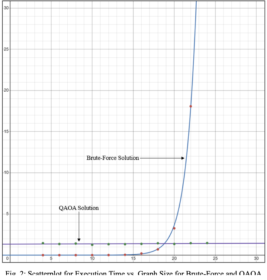
From the graph, it can be seen that the execution time for the brute-force solution shows exponential growth, whereas the execution time for the QAOA solution shows an almost flat linear model. At around 19 nodes, both algorithms’ average execution time curves intersect, after which the classical brute-force solution’s execution time exceeds that of the QAOA solution. This visual representation makes it even clearer how quickly the brute-force algorithm becomes more and more unscalable after a certain point, unlike the QAOA, which, although less accurate, seems to stay relatively constant regarding execution time. Note that the datapoint for ‘24 nodes’ for the brute-force solution is not shown as including it would make the fluctuations of the QAOA solution datapoints almost impossible to discern and the gap between both the curves before they intersect would be very small to see.

Discussion

This section analyzes the results obtained from the comparison between the classical brute-force algorithm and the QAOA in solving the Max-Cut problem. The discussion evaluates the observed trend between execution time and graph size for both algorithms, analyzes fluctuations and deviations from expected theoretical behavior, and explores the trend of the approximation ratio as graph size increases. It further investigates the causes of these trends, linking them to both algorithmic configurations and hardware limitations of the modern-day Noisy Intermediate-Scale Quantum (NISQ) devices (Mahmoud, 2021).

The execution time vs. graph size model derived from the data tables in the previous section shows a strong contrast between the trends of both algorithms. As expected, the classical brute-force solution shows an exponential growth in execution time as the number of vertices increases. This trend is consistent with the theory behind it, where every possible partition of vertices into two sets must be evaluated to deduce the optimal cut value. For small graphs (4–12 nodes), the execution time remains quite short, but as the graph size approaches 20–24 nodes, execution time grows dramatically due to the nature of an exponential function, quickly rendering brute-force computations infeasible on standard hardware. This rapid exponential escalation illustrates why NP-hard problems like the Max-Cut cannot have efficient classical solutions (solutions with polynomial time complexity), due to which they become completely infeasible for complex problems, underscoring the need for exploring quantum approaches that can theoretically have efficient solutions.

However, the QAOA solution displays a very different trend. Rather than growing exponentially with problem size, the execution times show an almost linear trend, fluctuating within a relatively narrow range, appearing almost constant across the entire set of tested graph sizes. This outcome contrasts that of QAOA (theoretically), which should show an approximately increasing linear trend with the number of qubits (and therefore graph size) increasing for a fixed circuit depth (p = 1) . The observed stability rather than increase and the randomness in runtime causing such fluctuations can be explained by a combination of quantum hardware behavior and implementation-level constraints. First, the QAOA code used in this experiment employs a fixed circuit depth and fixed Hamiltonian parameters γ = π/4 and β = π/2  . Because circuit depth, (consequently) gate count, and parameters remain constant, with no classical optimizer used to manipulate the parameters, the computational workload submitted to the 133-qubit ‘IBM_torino’ quantum device does not increase meaningfully with graph size within the tested range as there are enough qubits to encapsulate the entirety of the solution space all at once. The quantum processing time per circuit therefore remains nearly unchanged as graph size increases for those in the tested range, with small fluctuations attributable to backend scheduling variation, noise etc. In a practical setting, the Max-Cut problem is usually implemented with hundreds or even thousands of nodes, which are almost always greater than the qubit count, leading to increased processing time per circuit as graph size increases. Thus, under ideal, low-noise, and with a greater circuit depth, execution time of a QAOA solution could potentially consistently be observed to increase linearly with the number of qubits (and nodes on the graph) increasing on large and complex graphs.

Another key observation is regarding the approximation ratio. The experimental results show a decrease in approximation ratio of the QAOA solution as graph size increases. For small graphs, QAOA often seems to result in cuts close to optimal, but for larger graphs, its performance deteriorates slightly. In this investigation, this behavior can be caused by several factors. Firstly, with a low, fixed circuit depth  (p = 1) , the QAOA has a very low chance of providing a more optimal cut value due to the parameters not being optimized enough to lead to the Cost Hamiltonian’s application resulting in a higher measurement probability for bitstrings (basis states in the solution space) representing more optimal cut values. Thus, as the graph size grows, the solution space becomes exponentially greater, and a single-layer circuit cannot adequately explore it to favor bitstrings representing good cut values consistently. This is detrimental especially when the optimal cut corresponds to a low probability event. Secondly, the fixed parameter pair (γ = π/4, β = π/2) used in all runs, while simplifying the process, prevents dynamic tuning of the QAOA for different graph configurations, resulting in lower approximation ratios as the number of nodes (and therefore qubits) increases. Lastly, the most generic reason is noise. As the number of qubits used and operations performed increase, so does the capacity of noise in disturbing the compound quantum state the circuit is manipulating, blurring the probability distribution of basis states in the solution space, and therefore that of the measured bitstrings, resulting in suboptimal cut values.

Implications

This section considers the implications of the findings and discussions based on the previous sections for scalability of classical and quantum algorithms and when exactly does practical quantum advantage for NP-hard (optimization) problems such as Max-Cut begin to show. It then validates the viability of QAOA on modern NISQ hardware and considers the potential improvements that can be observed in the future as quantum hardware advances.

The findings presented in the previous sections demonstrate an important advantage of executing QAOA on real quantum hardware over the classical brute-force solution: while the latter method becomes rapidly infeasible to run with scale due to its exponentially increasing execution time, QAOA maintains roughly constant or at worst sub-linear growth in execution time. Although its current implementation does not achieve better speed compared to classical computation for relatively small graphs, its scalability over medium to large sized graphs suggests potential long-term advantages. However, the trend between graph size and approximation ratio observed proves to be a hurdle in the way of accuracy. The steadily declining approximation ratio shows the effect of QAOA configurations, but most importantly, noise. Even with a near-perfect QAOA algorithm, the limitations of NISQ hardware prevent the ability to create a high-depth circuit with a high qubit count without lowering accuracy due to the prevalence of noise. This prevents the observed advantages of QAOA for solving NP-hard problems from being effective where they are required the most – on large problems, and in the case of the Max-Cut problem, on large graphs, highlighting the underlying trade-off between speed and result accuracy

Conclusion

In summary, this investigation is designed to explore and demonstrate the feasibility of running QAOA for the Max-Cut problem on real quantum devices, comparing its performance against the classical brute-force method of solving the Max-Cut problem to gauge the potential advantages that quantum algorithms may provide as input size grows. The end goal is to determine when quantum algorithms start to outperform their classical counterparts.

The results from the experiment confirm that the classical brute-force algorithm scales exponentially with input size, becoming infeasible fairly quickly — over smaller graphs within the tested range, execution times were fairly short, but towards the end, execution times started to shoot upward at an alarmingly fast rate — whereas the QAOA solution had almost constant runtime for all graph sizes at the cost of accuracy as graph size increased. This limitation was shown by the decreasing average approximation ratio across all 5 trials as graph size increased, primarily due to a very low circuit depth (p >1)  , constant QAOA parameters, and most importantly, greater potential for noise on larger graphs, which is an issue for NISQ devices in general. Nevertheless, these findings validate the theoretical advantages that quantum algorithms outperform classical ones in terms of speed, but due to the shortcomings of NISQ hardware, they cannot fully be utilized for large problem sizes.

Ultimately, the insights from this investigation provide a foundation for understanding how quantum algorithms scale over problem size, bring us one step closer to realizing practical quantum advantages in solving complex NP-hard problems like Max-Cut over large problem sizes. Looking into the future, more advanced quantum hardware with larger qubit counts and lower noise levels will render increasing QAOA depth (p>1)  feasible with little effect on accuracy, allowing for faster and more accurate solutions for the Max-Cut problem and other NP-hard problems, revolutionizing areas such as semiconductor design, image segmentation in computer vision, financial modeling and data flow optimization, which use the Max-Cut problem for various purposes.

References

Agarapu, R. (2024). What is Hamiltonian in quantum mechanics? Online Tutorial Hub. Retrieved October 26, 2025, from https://onlinetutorialhub.com/quantum-computing-tutorials/what-is-hamiltonian-in-quantum-mechanics/

Algor Education. (n.d.). Brute Force Computing. Algor Education. Retrieved October 26, 2025, from https://cards.algoreducation.com/en/content/9CDDR2hL/brute-force-computing

Asfaw, A., Bello, L., Ben-Haim, Y., Bravyi, S., Capelluto, L., Carrera Vazquez, A., Ceroni, J., Gambetta, J., Garion, S., Gil, L., De La Puente Gonzalez, S., McKay, D., Minev, Z., Nation, P., Phan, A., Rattew, A., Shabani, J., Smolin, J., Temme, K., … Wootton, J. (n.d.). Learn Quantum Computing using Qiskit. Retrieved October 26, 2025, from https://github.com/RafeyIqbalRahman/Qiskit-Textbook/blob/master/Learn%20Quantum%20Computing%20using%20Qiskit.pdf

Bacon, D. M. (2003). Decoherence, Control, and Symmetry in Quantum Computers (Doctoral dissertation, University of California, Berkeley). arXiv:quant-ph/0305025. https://arxiv.org/pdf/quant-ph/0305025

Blekos, K., Brand, D., Ceschini, A., Chou, C., Li, R., Pandya, K., & Summer, A. (2023). A Review on Quantum Approximate Optimization Algorithm and its Variants. https://arxiv.org/pdf/2306.09198

Cai, J.-Y. (2003). Lecture 20: Goemans-Williamson MAXCUT Approximation Algorithm. University of Wisconsin-Madison. https://pages.cs.wisc.edu/~jyc/02-810notes/lecture20.pdf

Ceroni, J. (2025). QAOA introduction tutorial. PennyLane Quantum Machine Learning Demos. https://pennylane.ai/qml/demos/tutorial_qaoa_intro

Codecademy. (2022). Greedy algorithm explained. Codecademy. https://www.codecademy.com/article/greedy-algorithm-explained

Davis, R., Lanes, O., Waltrous, J. (2025). What is fault-tolerant quantum computing? Retrieved October 26, 2025, from https://www.ibm.com/quantum/blog/what-is-ftqc

DeepAI. (n.d.). Combinatorial optimization – machine learning glossary. DeepAI. https://deepai.org/machine-learning-glossary-and-terms/combinatorial-optimization

EITCA. (2024). In the context of QAOA, how do the cost Hamiltonian and mixing Hamiltonian contribute to exploring the solution space, and what are their typical forms for the Max-Cut problem? EITCA Academy. https://eitca.org/faq/in-the-context-of-qaoa-how-do-the-cost-hamiltonian-and-mixing-hamiltonian-contribute

Fiveable. (n.d.). Objective function. Retrieved October 26, 2025, from https://library.fiveable.me/key-terms/linear-algebra-and-differential-equations/objective-function

Goemans, M. X., & Williamson, D. P. (1995). Improved approximation algorithms for maximum cut and satisfiability problems using semidefinite programming. Journal of the ACM, 42(6), 1115–1145. https://math.mit.edu/~goemans/PAPERS/maxcut-jacm.pdf

Preskill, J. (2018). Quantum Computing in the NISQ era and beyond. Quantum, 2, 79. https://quantum-journal.org/papers/q-2018-08-06-79/pdf/

Ivezic, M. (2024). Quantum Approximate Optimization Algorithm (QAOA). Retrieved October 26, 2025, from https://postquantum.com/quantum-computing/quantum-approximate-optimization-algorithm-qaoa/

Jaillet, P. (2010). NP-completeness. MIT 6.006: Introduction to Algorithms. Retrieved from https://courses.csail.mit.edu/6.006/fall10/lectures/lecture24.pdf

Kanwal, A. (2021). Understanding P, NP, NP-complete, and NP-hard problems: A fundamental guide. Medium. https://medium.com/@0ayesha.kanwal/understanding-p-np-np-complete-and-np-hard-problems-a-fundamental-guide-3924fc9ece2a

Lee, J. (2010). A first course in combinatorial optimization. Cambridge University Press. https://books.google.com.tr/books?id=3pL1B7WVYnAC&pg=PA1&redir_esc=y#v=onepage&q&f=false

Lotshaw, P. C., Nguyen, T., Santana, A., McCaskey, A., Herrman, R., Ostrowski, J., Siopsis, G., & Humble, T. S. (2022). Scaling quantum approximate optimization on near-term hardware. Scientific Reports, Nature Publishing Group. https://www.nature.com/articles/s41598-022-14767-w

Luca, G. D. (2023). Introduction to graph theory. Baeldung on Computer Science. https://www.baeldung.com/cs/graph-theory-intro

Mahmoud, A. (2021, June 27). What is Quantum Computing? https://www.techspot.com/article/2280-what-is-quantum-computing

Maltby, H., & Ross, E. (n.d.). Combinatorial optimization. Brilliant. https://brilliant.org/wiki/combinatorial-optimization

Rossi, M., Cohen, S., & Smith, J. (2024). What is Quantum Parallelism, Anyhow?. https://arxiv.org/html/2405.07222v1

Swayne, M. (2024). Quantum computing challenges. https://thequantuminsider.com/2023/03/24/quantum-computing-challenges/

Tepanyan, H. (2025). Quantum Computing vs. Classical Computing. Retrieved October 26, 2025, from https://www.bluequbit.io/quantum-computing-vs-classical-computing

Thomson, J. (2025). What is quantum superposition and what does it mean for quantum computing? Retrieved October 26, 2025, from https://www.livescience.com/technology/computing/what-is-quantum-superposition-and-what-does-it-mean-for-quantum-computing

Toni, B. (2018). Max-Cut lecture notes (PDF). University of Toronto. http://www.cs.toronto.edu/~toni/Courses/Proofs-SOS-2018/Lectures/maxcut.pdf\

Viana, P.A., Neto, F. (2024). Quantum search algorithms for structured databases. https://arxiv.org/pdf/2501.01058

Wright, S. J. (2025). Optimization Definition, Techniques, & Facts. Encyclopaedia Britannica. https://www.britannica.com/science/optimization

Data and code used in this paper are available in github.

---