

Author: Aman Kumar
Mentor: Dr. Osman Yagan
Wayland High School
Abstract
Multi-armed bandit algorithms are decision-making algorithms that select between a set of options a specified number of times. Each option, or arm, has a specified, fixed cost and gives a reward which is randomly sampled from a fixed distribution. There exists an optimal action to take, which is choosing the cheapest arm which gives a reward above the predetermined threshold. Choosing a suboptimal arm can lead to cost regret, reward regret, or both. The function of the algorithm is to minimize these regrets. The combinatorial variation of bandits allows for the selection of multiple arms in a single round, whose costs and rewards are averaged. This can potentially lead to lower regrets and higher efficiency. This paper investigates the different parameters of the combinatorial cost-subsidy bandit algorithm and determines its effectiveness. These parameters are tested in several experiments run in VSCode using the MovieLens 25M dataset.
Keywords: Arm, cost, reward, cost regret, reward regret, round, threshold, horizon, logarithmic, combinatorial
Introduction
At its core, a multi-armed cost-subsidy bandit algorithm contains a horizon, a threshold, and a set of arms, each with its own cost and reward distribution (Juneja et al., 2025). The horizon gives the desired number of rounds, and in each round, the algorithm selects an arm (or multiple, in the case of a combinatorial bandit). The threshold gives the desired reward from the selected arm(s). Based on this threshold, an optimal cost is calculated, using the mean rewards of each arm. This optimal cost represents the cheapest arm or combination of arms that will meet the reward threshold. This is then used in the calculation of the cost regret. Each round, if the cost of the selected arm(s) is larger than the optimal cost, the difference is added to the total cost regret. With a horizon of n, a cost during round t of ct, and an optimal cost of c*, this can be represented as follows (Juneja et al., 2025):
The reward regret is calculated using the threshold. Each round, if the mean reward of the selected arm(s) is smaller than the threshold, the difference is added to the total reward regret. It is important to note that it is the mean reward that is considered, not the reward achieved in the particular round. With a horizon of n, a threshold of μ*, and a reward during round t of μt, this can be represented as follows (Juneja et al., 2025):
The purpose of the algorithm is to minimize these two quantities. Several different types of bandits achieve this in different ways, but the one used in this paper uses the upper confidence bound (UCB) method. It begins by selecting each arm once and keeping track of the received rewards. Each round after this, it selects the cheapest arm that has reasonable potential to be at or above the threshold. The potential of each arm, also known as its UCB index, is calculated by adding a confidence term to the average reward received from its prior results (Lattimore & Szepesvári, 2020). It is the upper limit of a confidence interval on its mean reward. This term is dependent upon the max difference in potential rewards across the dataset, which in the case of the movielands set, is 4. It is also dependent on the number of times the specified arm has been selected. With a horizon of n, a max difference of Δr, and the number of times a given arm i has been selected by round t of Ti(t), this can be represented as follows (Ganesh, 2019):
The equation contains a constant l, which can be varied, usually in the range 1-4. If multiple arms are being averaged together, each individual upper bound is used. As an arm is selected more times, its interval narrows, as there is more certainty around its expected value. The algorithm learns and improves over the rounds, and it results in the total regret graphs taking a logarithmic shape.
One of the most beneficial aspects of using a bandit algorithm is that it gives each arm the chances it deserves; no more, no less. If a person was manually making decisions based on rewards, they may neglect arms which initially failed to offer satisfactory returns. However, because each arm has a UCB index which is inversely proportional to the number of times it has been pulled, it can still be chosen even if it has a bad start. If it continues to disappoint, it will be phased out, but if it turns around, it can potentially provide value.
Combinatorial bandit algorithms allow for the selection of multiple arms in a single round (Xu & Li, 2021). The weighting of each arm can be varied, but this paper will use a uniform average.
The goal of this paper is to test the combinatorial cost-subsidy bandit algorithm. The effect of changing the parameter l will be tested. Additionally, the effectiveness of using multi-arm solutions will also be tested. This will be done by using a specific set of costs whose optimal solution requires multiple arms and seeing how the algorithm improves when it is allowed to use more arms.
Method
The experiment is conducted using the Movielands 25M dataset, which contains ratings of movies of 19 different genres. A cost is assigned to each genre for the experiment. The genres, mean ratings, and costs are shown in the following table:
The first aspect to be tested is the effectiveness of using multi armed solutions. This will be tested by running the algorithm on three settings: one arm allowed, two arms allowed, and three arms allowed. For each setting, it will be run 100 times, and the results will be averaged. For this experiment, the reward threshold is the average rating across the entire set, which is 3.6251287887254984. Using this table of costs, the optimal cost for this threshold using only one arm is 0.71, which is the crime genre. However, the optimal cost goes down when two arms can be selected and averaged. It goes to 0.625, which is the average of the crime and thriller genres. When it is further increased to three selected arms, the optimal cost drops to 0.6, which is the average of the crime, thriller, and romance genres. 0.6 will be used as the optimal cost for all three settings in order to test if the three arm setting can do better than the two and one arm settings.
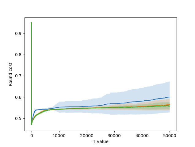
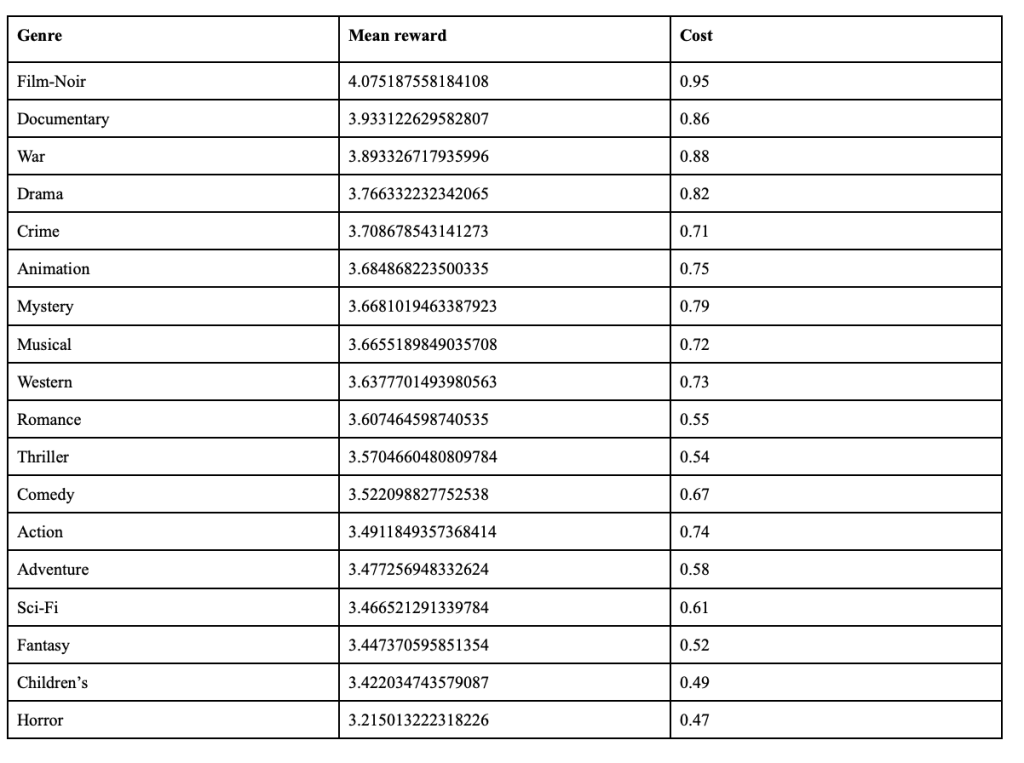
Figure 1 – Round-by-round cost for each setting.
Figure 1 shows the graph of the round-by-round cost for each setting. The one-arm setting is blue, the two-arm setting is orange, and the three-arm setting is green. The shaded regions represent the range created by adding and subtracting one standard deviation from the means. The one-arm setting is significantly above the other two, which was expected given that its optimal cost was much higher. The two and three-arm settings are very close together, though there is some difference, especially towards the end. The three-arm setting can find an optimal combination, while the two-arm setting is unable to.
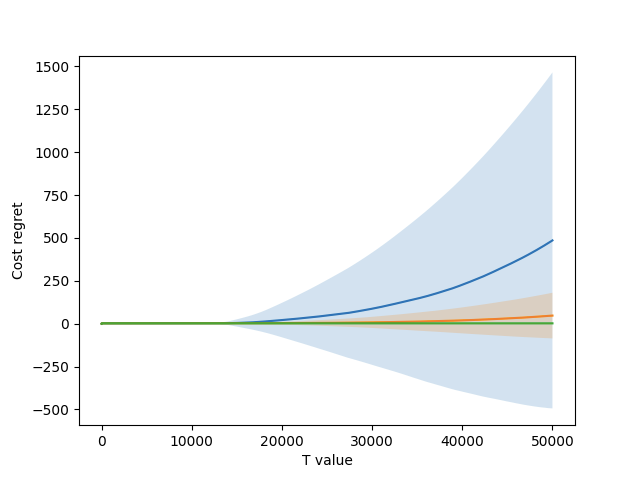
Figure 2 shows the graph of the cumulative incurred cost regret for each setting. All three settings can stay under the optimal cost at the start, as they have more options to choose from due to the confidence bounds being so wide. However, as these bounds narrow and the true value of each arm becomes more apparent, the one-arm and two-arm settings start to incur regret. However, the three-arm setting can stay flat, as it has access to the optimal combination. Overall, the one arm setting incurred an average of 485.6 cost regret by the end, the two arm setting incurred 47.3, and the three arm setting incurred just 2.0.
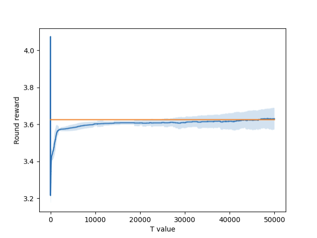
Figure 3 – Round-by-round reward for 1 arm setting.
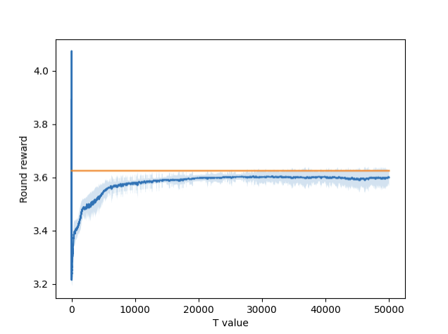
Figure 4 – Round-by-round reward for 2 arm setting.
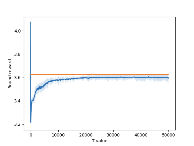
Figure 5 – Round-by-round reward for 3 arm setting.
Figures 3, 4, and 5 show the graphs of the round-by-round rewards for each setting. Included in each graph is the threshold, represented by the orange line. The single arm setting performs slightly better, while the double and triple are a little behind. This is likely because the single arm setting has fewer overall options to choose from, meaning there are fewer suboptimal solutions to fool it.
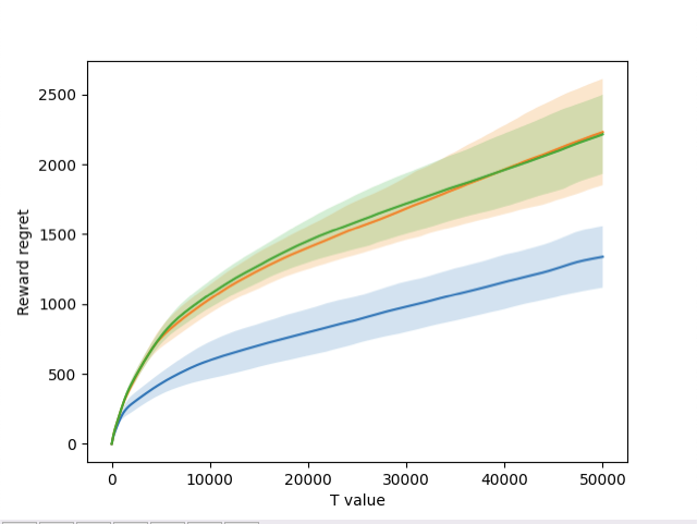
Figure 6 – Total incurred reward regret by round for all settings.
Figure 6 shows the graph of the cumulative incurred reward regret for each setting. Once again, the one-arm setting is blue, the two-arm setting is orange, and the three-arm setting is green. The two-arm and three-arm settings performed extremely similarly, finishing with regrets of 2232.1 and 2216.2, respectively. The one-arm setting was more effective, finishing with a regret of 1338.9. All three settings were able to learn and improve across the horizon, and were able to achieve the desired logarithmic shape.
Overall, the three-arm setting incurred a reward regret that was 99.2% of the two-arm setting and 165.5% of the one-arm setting. However, it was extremely effective in cost, as it incurred a cost regret that was 4.2% of the two-arm setting and 0.4% of the one-arm setting.
The second parameter to be tested is the l value. As mentioned in the introduction, the l value is a factor in the calculation of the confidence bounds around each arm’s expected reward. The three values of l that will be tested are 1, 2, and 4. Once again, 100 experiments will be run and averaged with each setting, and one standard deviation above and below the mean will be shaded on the graph.
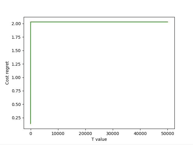
Figure 7 – Total incurred cost regret by round for all settings.
Figure 7 shows the graph of the cumulative incurred cost regret for each l value. All three are exactly the same, accumulating regret during the initial exploration phase before staying flat the rest of the way. This was expected, as these experiments were run using the three-arm setting, which is extremely effective in minimizing cost regret.
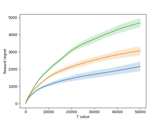
Figure 8 – Total incurred reward regret by round for all settings.
Figure 8 shows the graph of the cumulative incurred reward regret for each l value. This graph is more varied. The blue represents an l value of 1, the orange represents an l value of 2, and the green represents an l value of 4. The results show that all three l settings are able to learn and improve, but an l value of 1 performs the best. In general, a lower l value is better, as larger values give too wide estimates for the rewards of the arms. However, if it goes too low, then an optimal arm may not get chosen after a few pulls if it gives suboptimal results.
Conclusion
The results of this paper show that the combinatorial bandit algorithm is extremely cost-effective in decision making. While it gives up a little bit in terms of rewards, it makes up for it by reducing the costs.
The algorithm can be utilized in any situation with decisions involving costs and rewards. For example, in the context of the dataset used in this paper, the algorithm can be used to choose movies to show to audiences. Each arm can be a genre, and the playing of a movie of the genre represents the pulling of the arm. The rewards are the reviews, and using these reviews, the algorithm can decide which movies to show. It can also be used in an educational setting. Each arm can be a specific lesson plan or style, and rewards can be test scores, student feedback, or another evaluation metric. Using the evaluations, the algorithm can decide the most effective lessons to teach.
A further direction for exploration could be the testing of an algorithm that can pull multiple arms with different weights. Instead of simply averaging them out evenly, it could take more from one and less from another. This could potentially allow for even better combinations of arms.
Bibliography
Lattimore, Tor and Szepesvári, Csaba. “Bandit Algorithms.” Cambridge University Press, 2020
Juneja, Ishank, et al. “Pairwise Elimination with Instance-Dependent Guarantees for Bandits with Cost Subsidy.” International Conference on Learning Representations, 2025
Ganesh, A.J. “Multi-armed Bandits.” University of Bristol, 2019
Xu, Haike and Li, Jian. “Simple Combinatorial Algorithms for Combinatorial Bandits: Corruptions and Approximations.” Institute for Interdisciplinary Information Sciences (IIIS), Tsinghua University, 2021
About the author
Aman Kumar
Aman is a high school senior studying at Wayland High School in Massachusetts. He is interested in math, computer science, and data science. Outside of academics, he plays the clarinet, and is a big football fan, supporting the New England Patriots.