

Author: Rohaan Narula
Mentor: Dr. Ella Atkins
King’s College School, Wimbledon
Abstract
Solar-powered unmanned aerial vehicles (UAVs) carry no fuel, meaning their endurance is governed by a balancing act crafted between the energy harvested from sunlight and the energy consumed throughout flight, rather than conventional fuel capacity constraints. Over multi-day missions, this balance becomes hard to predict, as solar harvesting depends on the Sun’s position relative to the UAV whilst energy consumption depends on the aerodynamic forces required to sustain flight. Both of these are also affected by flight conditions and cruise altitudes, meaning a complex optimisation problem emerges. Many simplified models treat the Sun as stationary, an assumption only valid for short missions over small timeframes and distances. In this paper, solar harvesting will be modelled through a fixed panel and gimballed panel approach, where a gimballed panel traces the Sun’s position relative to the UAV and points the panel at the optimal orientation for maximum irradiance.
Overall, this paper develops a model that investigates the energy balance aforementioned, using the example of a transatlantic crossing from London to New York. There are three overarching MATLAB models that are integrated into this energy balance: great-circle navigation, aerodynamic power consumption, and solar energy harvesting. The flight parameters have been derived from steady-level flight mechanics, standardised NACA tables, photovoltaic conversion data and solar geometry.
Having completed the simulations, it can be seen that an idealised gimballed solar panel increases total harvested energy substantially, by 62%, but much of the additional energy that it harvests cannot be stored, since the battery charge is already full during daylight hours, where there is peak harvesting. This is shown as the minimum state-of-charge only increases by 5% for a gimballed panel, starkly lower than the 62% rise in energy harvesting aforementioned. As a result, it can be said that endurance in this context cannot be governed solely by aerodynamic efficiency or solar collection gains, but by the capacity of the battery to carry energy across extended periods of insufficient insolation.
Future work on this issue should therefore treat battery capacity as a design variable to be considered alongside altitude and cruise conditions, whilst also relaxing assumptions discussed throughout. This concept has potential real-world applications in wildfire monitoring, surveillance/law enforcement, shipping, and ocean monitoring.
1. Introduction
1.1 Motivation
Solar-powered unmanned aerial vehicles (UAVs) offer the ability of extremely long endurance without the constraints provided by conventional fuel. Their endurance is governed simply by the balance and optimisation between the electrical energy harvested by the sun, and the energy consumption by the UAV in flight. As a result, solar flight is attractive for a multitude of applications that require persistent operation, over large and remote areas. Such examples include maritime search and rescue, wildfire detection and atmospheric surveying in remote areas. This concept has been demonstrated experimentally before, with AtlantikSolar achieving an 81-hour continuous flight.(Oettershagen, et al., A solar-powered hand-launchable UAV for low-altitude multi-day continuous flight, 2015)(Oettershagen, et al., Design of small hand-launched solar-powered UAVs: From concept study to a multi-day world endurance record flight, 2017) The concept explored in this paper also explores the idea of a moveable (on the pitch and roll axis) solar panel on the UAV, allowing it to maximise the electrical energy it harvests from the sun, a concept yet to be quantified by existing studies. The primary reason this has not been integrated into mainstream UAV technology is due to the aerodynamic and mass penalties of such a gimbal system, which are noted as limitations throughout.
In general, the primary difficulty with a solar-powered UAV tends to be that the energy balance of the UAV is directly proportional to the aircraft’s flight conditions and environmental. Solar collection also depends on the position of the sun relative to the aircraft (with a non-gimballed system), which varies with latitude, time of day, and season. Furthermore, aircraft energy consumption varies on the aerodynamic forces required to maintain steady-level flight in a cruise state. These forces vary significantly with changes in airspeed, air density, and lift coefficient, with air density itself varying with altitude. Consequently, due to the balancing act of these two factors, one cannot simply consider aerodynamic or solar conditions alone, creating a complex problem.
Multiple attempts have been made to simplify or solve this problem, with some choosing to limit mission distance and time as being short relative to the sun’s position, allowing it to be treated as stationary. (Klesh & Kabamba, 2009)Others provide validated airframes and power-collection models but lack investigation into cruise-altitude or even route optimisation for a multi-day mission. (Oettershagen, et al., A solar-powered hand-launchable UAV for low-altitude multi-day continuous flight, 2015)The trade-off between altitude, flight conditions, and battery margin over a multi-day mission therefore remains unestablished, and this paper attempts to address this gap.
2. Preliminaries
2.1 Steady Level Flight
The aircraft is modelled in steady, level cruise. This is primarily due to time constraints and aerodynamical complexities involved in take-off, climb, descent and landing phases, which could further complicate the solar harvesting model mentioned later on. The diagram below contains four forces acting in the aircraft’s x-z plane: lift perpendicular to the flight path, drag opposing the direction of motion, thrust along the flight path, and weight acting vertically downwards.
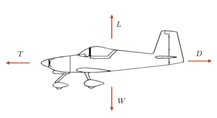
Figure 1 – Forces Acting on Aircraft in Steady-Level Flight
Steady level flight involves no acceleration, so these forces balance in pairs:

Together, these two conditions establish the relationship between airspeed, lift coefficient and altitude: once aircraft parameters are established, the air density at a given altitude details the airspeed required at a chosen lift coefficient. (Fidowski, Atkins, & Powell, 2019)(Anderson, 1999)
The equations for lift and drag forces are given by Equation [2] below:

Here, V is true airspeed, ρ air density, S is the wing reference area over which airflow occurs, and CD and CL are drag and lift coefficients. The quantity 1/2 ρV2 therefore describes the dynamic pressure. (Fidowski, Atkins, & Powell, 2019)
If we combine Equation [2] with the lift-weight balance condition in Equation [1], we get the following, Equation [3], the airspeed required to sustain a specified lift coefficient at a particular altitude:

The aerodynamic coefficients are derived from two-dimensional NACA 4415 section data. (Abbott & von Doenhoff, 1959)(Airfoil Tools, n.d.) NACA 4415 was selected due to its combination of lift-to-drag performance and sufficient thickness to accommodate both solar-cell installation and endurance structural requirements. We can calculate the Reynold’s Number of the aerofoil using Equation [4] below:

At this Reynolds number the section lift curve is markedly non-linear: the local slope falls from approximately 0.21 per degree near zero incidence to 0.06 per degree at eight degrees, a consequence of a laminar separation bubble whose extent varies with incidence. A single linear fit is therefore not representative, and the tabulated section data are used directly rather than through a lift-curve slope approximation. The drag polar is obtained by fitting the drag coefficient against the square of the lift coefficient over the same data, which does not require the lift curve to be linear. (Airfoil Tools, n.d.)(Drela, 1989)
The two-dimensional data are then corrected for a finite wing. A real wing sheds tip vortices, which induce a downwash and generate induced drag proportional to the square of the lift coefficient. The downwash also reduces the effective angle of attack seen by the section, so the geometric angle of attack required to achieve a given lift coefficient exceeds the two-dimensional value by the induced angle. (Anderson, 1999)
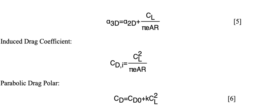
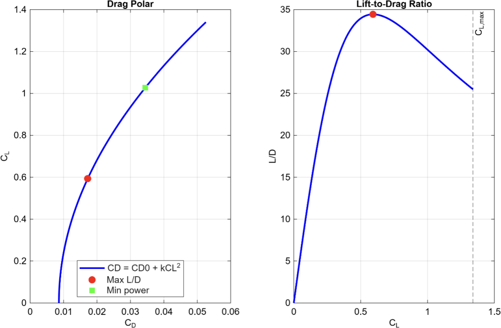
InFor this model, there are two relevant aerodynamic operating points. The first is maximum lift-to-drag ratio, which can be calculated by differentiating with respect to and setting the derivative equal to zero. (Fidowski, Atkins, & Powell, 2019) This can be seen below in Eq. [7].

This condition occurs when parasitic drag and induced drag are equal. This is at CL = 0.593, kC2L = 0.00861, matching CD0 exactly. The condition also occurs at minimum power, given by Eq. [8]:
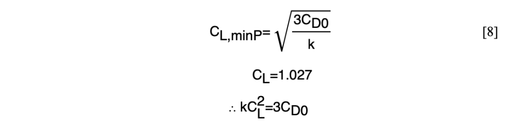
Here, at the minimum power condition we can see that induced drag is three times the parasitic drag. This is because power is the product of the drag and airspeed, so the additional velocity dependence causes the optimum condition to be shifted to a higher lift coefficient.
The difference between these operating conditions matters for a long-duration solar flight, as maximum L/D ratio would minimise drag and therefore the energy required over a fixed distance. Since that energy is the product of the drag and the distance flown, it corresponds to a maximum range condition. On the other hand, minimum power minimises the electrical demand at each instant and therefore corresponds to a maximum endurance condition.
Figure 2 demonstrates the comparison between maximum L/D ratio and minimum power utilising the flight parameters of our aircraft that can be found in the Appendix.
2.2 Standard Atmospheric Conditions
Air density will vary significantly across the altitude range considered. A function of air density as altitude varies can be obtained, combining the hydrostatic relationships and ideal gas laws with a linear temperature profile in the troposphere. This is given in Eq. [9] and [10] below:
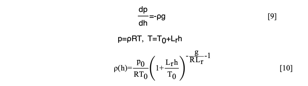
The constants in the equations above are:

(International Organization for Standardization, 1975)
This model is valid up to 11km altitude. This function is utilised to calculate the airspeed required to generate lift at different altitudes, as when density falls, the aircraft must fly faster to generate the same lift at a given lift coefficient, changing the power required.
2.3 Propulsion
For a propellor-driven aircraft, electrical power is the most useful measure to determine energy consumption. This is because the battery energy balance depends on the electrical consumption of the propulsion system. Eq. [11] gives the propulsion model, combining aerodynamic power requirements with the propulsion efficiency nprop and the constant avionics load Pav . (Fidowski, Atkins, & Powell, 2019)

2.4 Solar Position
The solar power available to harvest by the aircraft is set by the irradiance incidence on the illuminated panel area, and the conversion efficiency of the photovoltaic system. Irradiance will vary continuously with geographic position, time of day, season, and altitude, so solar harvesting must be evaluated along the trajectory of its transatlantic route, rather than being treated as a constant power source.
The Sun’s position relative to the aircraft follows from the solar declination angle, the aircraft latitude, and the solar hour angle. (Duffie & Beckman, 2013)(Cooper, 1969) For a day of year , the declination can be approximated through the following equation:

The hour angle follows from local solar time, with H = 0 at solar noon:

The solar elevation above the local horizontal can therefore be given through the spherical law of cosines, applied to the triangle formed by the pole, aircraft zenith, and the Sun:

Here, is the aircraft latitude. Eq. [14] is the same as computing the great-circle central angle between the aircraft and the subsolar point, since the hour angle is the longitude difference between them.
2.5 Atmospheric Attenuation
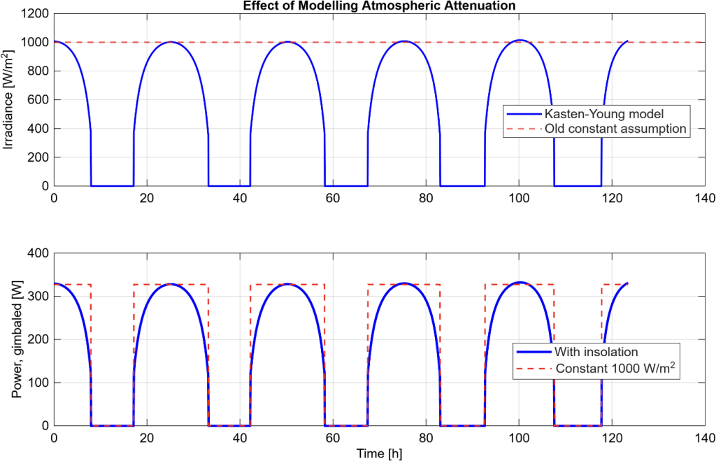
The irradiance reaching the aircraft is also reduced by absorption and scattering across the atmospheric path, and as the Sun sits lower throughout the day, the longer that atmospheric path becomes. The relative optical air mass can be approximated using the Kasten-Young formulation, which accounts for atmospheric curvature, and remains finite at the horizon. (Kasten & Young, 1989)

Flying at altitude also reduces the mass of atmosphere above the aircraft, which can be accounted for by scaling the air mass by the local pressure ratio from the standard atmosphere model described in Section 2.2. The direct normal irradiance then can be placed in an empirical clear-sky attenuation model:
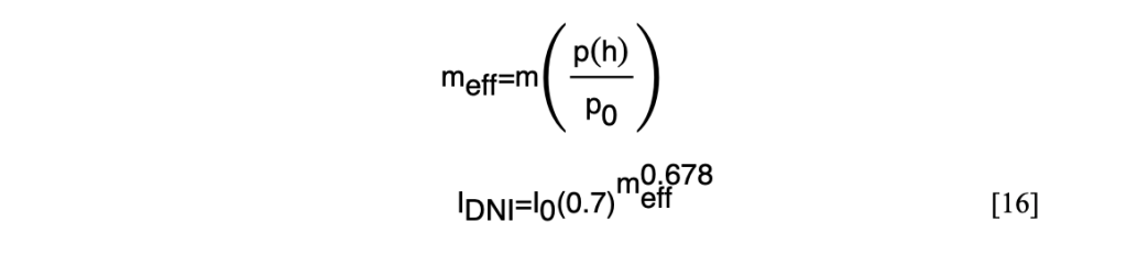
Here, I0 = 1361 Wm-2 is the solar constant, and the coefficient 0.7 corresponds to the fraction transmitted at unit air mass. (Meinel & Meinel, 1976) The exponent 0.678 is an empirical fit accounting for non-uniformity in the distinct atmospheric layers. This model captures both the reduction in available energy as the Sun approaches the horizon and the increase in irradiance at higher cruise altitudes. Diffused and ground-reflected components of irradiance have been assumed to be negligible as part of this investigation.
Figure 3 demonstrates the effects of the differing insolation models.
2.6 Photovoltaic Conversion
The electrical power generated from an illuminated panel is:

Where APV is the photovoltaic cell area, ηPV the module conversion efficiency, ηPMMT the efficiency of the maximum-power-point tracking electronics, and the angle between the solar direction and the panel normal. For the aircraft considered in this paper, APV = 1.7223 m2 , as it has been taken as equal to the wing planform area. Furthermore, ηPV = .2 and ηPMMT = .95. The conversion process is entirely independent of flight conditions, so variation in harvested power arises entirely from solar geometry and atmospheric attenuation. (Duffie & Beckman, 2013)(Oettershagen, et al., A solar-powered hand-launchable UAV for low-altitude multi-day continuous flight, 2015)
3. Methods
The following sections detail the mathematics behind MATLAB models utilised in this study. Access to these models can be found through the GitHub repository linked here:https://github.com/rohaannarula/solar-uav-energy-model
3.1 Panel Orientation & Solar Collection
The incidence angle, ɸ introduced in Eq. [17] follows from the relative orientation of the Sun and the solar panel. Both directions are represented as unit vectors in a local North-East-ηPV (NED) frame. (Fidowski, Atkins, & Powell, 2019) The solar direction is:

Here, a is the solar azimuth, measured clockwise from North, and θs is the solar elevation. The negative third component is due to the downwards axis being positive, so the Sun above the horizon has a negative vertical component. For a panel with roll angle ɸp and pitch angle θp , with yaw fixed at zero, the outward normal is:

Because both of these vectors have unit length, their dot product gives the cosine of the incidence angle directly. The result is fixed above zero, since a negative value implies the Sun lies behind the panel, and no energy is collected:

Two configurations will be evaluated. The first is a flat panel, representing the roughly horizontal photovoltaic surface of an aircraft in steady-level cruise. At a maximum lift-to-drag condition, the required lift coefficient of 0.593 is established using an average cruise angle of 1.11°. This is close to the horizontal, making a flat panel assumption reasonable. Setting both orientation angles to zero reduces Eq. [20] to exactly the sine of the solar elevation:

The second configuration is an idealised gimballed panel; tracing the Sun’s position. The required orientation is obtained by equating the panel normal to the solar direction, which yields three separate component equations into two unknowns. The East component contains the roll angle and yields the pitch by dividing the North component by the Down component, which eliminates the roll term.

Two angles are enough for the three equations because the solar direction is a unit vector, so only two of its components are independent of each other. The yaw angle does not appear, as rotating the panel about its own axis does not alter the theoretical solar panel surface presented to the Sun.
In both configurations, the harvesting of solar energy is reduced significantly when solar elevation is below 5º , at which point the atmospheric path length is long enough that available irradiance becomes negligible. The gimballed panel can be treated as an idealistic case, rather than a realisable configuration, due to multiple assumptions required, such as the requirement for near vertical pitch near sunrise and sunset.
3.2 Great-Circle Route
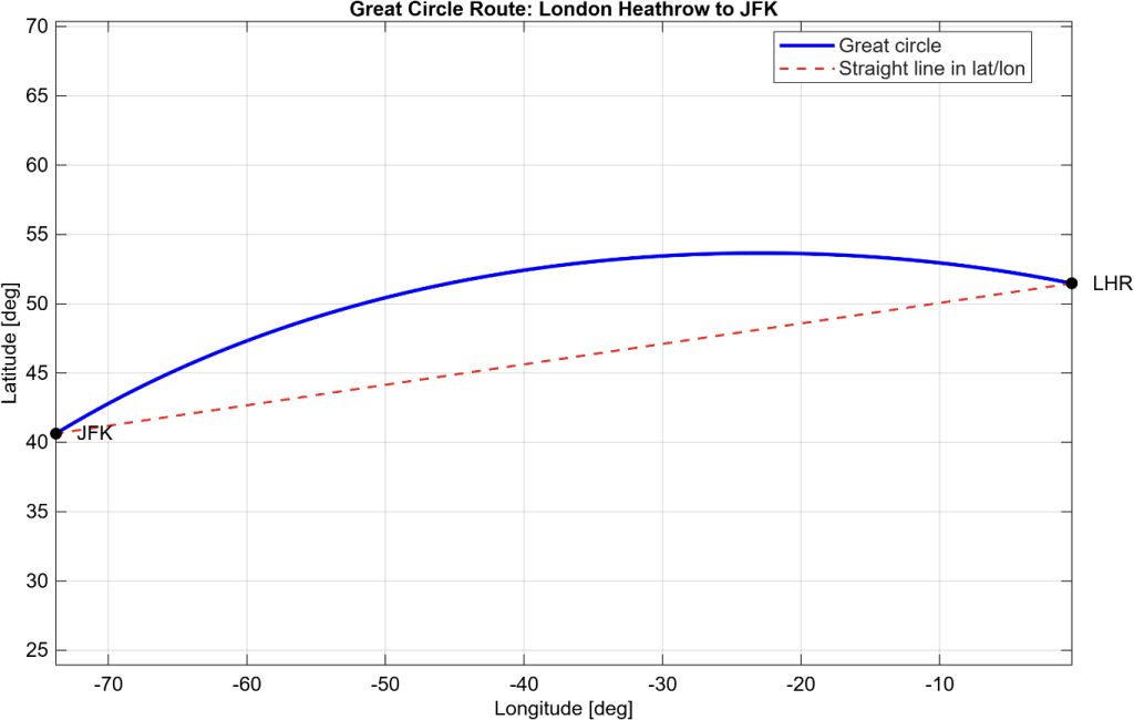
The aircraft must follow the shortest possible path between London Heathrow and John F. Kennedy International Aiport on a spherical Earth, which is a great-circle arc. For endpoint co-ordinates with longitude difference Δƛ , the central angle subtended at the Earth’s centre is as follows:

As a result, the great circle distance and initial heading can be calculated, where is the radius of the Earth:

A four-quadrant arctan2 function can be used throughout, in place of a simple arctan one, since dividing the sine and cosine components would discard their individual signs and therefore lose the directional element of the heading.
As great-circle routes do not maintain constant heading, the aircraft heading will change continuously throughout crossing. Intermediate vectors can be generated through spherical linear interpolation, where is the fractional distance along the route, and and are unit position vectors:

The result can then be converted back into latitude and longitude for the solar and atmospheric calculations. The route is decomposed into 2000 equally spaced points and is plotted below in Figure 4.
3.3 Cruise State & Energy Balance
For each cruise altitude and flight condition, the energy balance model is calculated independently. Utilising parameters obtained from Section 2; we can calculate the required electrical power and flight time:

Where Pelec is the required electrical power for a given altitude and flight condition.
We can calculate solar power required using the trapezium rule, as solar power harvested varies with both time and position, and is continuously varying:

The battery can be represented as an energy reservoir with limited capacity, updated according to the net electrical power balance:

Where EB max = 850 Wh = 3.06MJ and the battery is initially fully charged. (Oettershagen, et al., A solar-powered hand-launchable UAV for low-altitude multi-day continuous flight, 2015) We can therefore calculate the state of charge, and the aircraft’s minimum state of charge over the flight:

The minimum state of charge is utilised as the primary measure of mission feasibility, as it is more informative than comparing net energy expenditure. This is because a positive net balance will not guarantee that sufficient energy is available throughout the flight.
The simulation of state of charge will be repeated for each altitude, with both cruise conditions and panel configurations. I will consider a minimum SOC requirement of 30% to consider feasibility, as assumptions discussed later diminish true viability of such a large margin.
4. Results
4.1 Solar Collection
The great-circle route from London Heathrow to JFK New York spans 5540km. If the aircraft departs at 12.00 UTC on day 172 of the year, close to June solstice, the crossing at an altitude of 3000m encompasses 5 whole day-night cycles.
Figure 5 compares solar power generated by the flat and idealised gimballed configurations. Peak values appear similar, approximately 329W when gimballed against 291W, but the gimballed curve is broader, unlike the narrow daily peak of the flat configuration. Integrated across the crossing, at maximum L/D ratio, the two configurations collect 77.37MJ and 48.17MJ respectively, so continuous gimballed tracking yields 62% more energy harvested. The differences arise at low solar elevation, where a flat panel projects only 50% of the direct beam at 30 degrees and 17% at 10 degrees, compounding the atmospheric attenuation already present. This is represented by Figure 5.
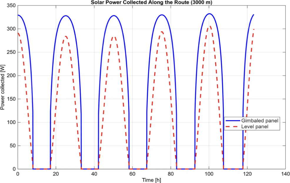
Figure 5 – Solar Power Harvesting Comparison
4.2 Battery State-of-Charge
Figure 6 below shows the battery state of charge over the same crossing. The battery reaches full capacity for several hours each day, meaning surplus energy harvested cannot be stored given current battery size constraints. Approximately 26.1 MJ is discarded across the maximum-L/D mission, exceeding the 22.02 MJ required to complete the crossing. Storage rather than collection is therefore the binding constraint, and the additional energy gathered by the gimballed panel does not translate proportionally into endurance. The minimum state of charge is a more useful measure of feasibility than net energy balance, as explained in section 3.3.
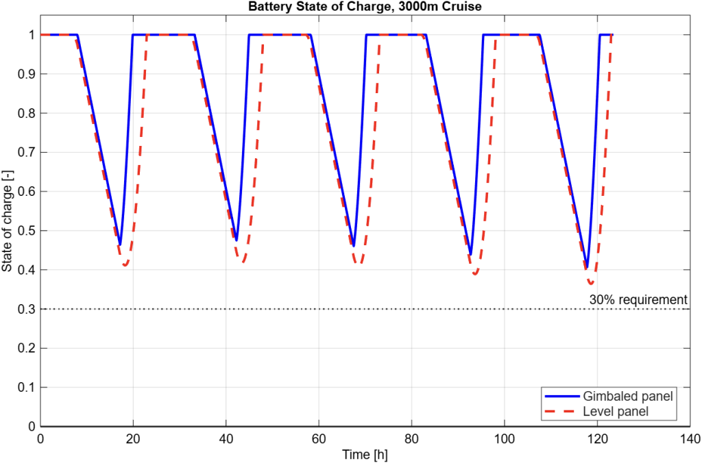
Figure 6 – Battery State of Charge Across Flight
4.3 Panel Orientation
According to simulation, the ideal orientation requires panel roll to sweep between approximately ±60° each day and pitch to reach nearly −80° near sunrise and sunset, a range no practical mechanism could achieve, reinforcing the treatment of the gimballed case as an upper bound. The photovoltaic panel parameters can be found in the Appendix.
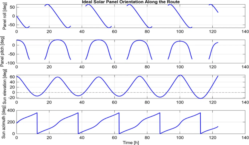
Figure 7 – Panel Orientation Across the Route
4.3 Effect of Cruise Altitude and Flight Condition
| Altitude [m] | Condition | Velocity [m/s] | Power Req. [W] | Time [h] | Energy Req. [MJ] | Average Harvest rate [W] | SOCmin | SOCmin Gimballed |
| 0 | Max L/D | 10.74 | 43.31 | 143.3 | 22.34 | 95.4 | 0.437 | 0.481 |
| 0 | Min power | 8.16 | 38.55 | 188.6 | 26.17 | 97.7 | 0.516 | 0.551 |
| 3000 | Max L/D | 12.47 | 49.55 | 123.4 | 22.02 | 108.4 | 0.365 | 0.410 |
| 3000 | Min power | 9.47 | 44.03 | 162.5 | 25.75 | 109.7 | 0.454 | 0.491 |
| 6000 | Max L/D | 14.63 | 57.39 | 105.2 | 21.73 | 127.8 | 0.275 | 0.322 |
| 6000 | Min power | 11.12 | 50.90 | 138.4 | 25.36 | 119.6 | 0.374 | 0.411 |
| 10000 | Max L/D | 18.50 | 71.37 | 83.2 | 21.37 | 142.2 | 0.102 | 0.221 |
| 10000 | Min power | 14.06 | 63.17 | 109.5 | 24.89 | 137.2 | 0.218 | 0.259 |
Table 1 above summarises the design variables. The energy required falls only 4.3% across the entire altitude range, because drag at fixed is independent of air density. On the other hand, battery margin falls much more sharply, from 0.437 to 0.102 under maximum L/D ratio, since greater altitudes raises power required from 43.3 to 71.4 W while night duration is unchanged. The 30% SOC requirement is only met to approximately 5 km. In terms of flight condition chosen; maximum L/D ratio consumes 15 percent less energy at every altitude, while minimum power leaves a larger reserve because it draws less overnight. This disparity grows with altitude, and at 6000m maximum L/D fails the margin requirement at 0.275 while minimum power satisfies it at 0.374. However, maximum L/D has immense benefits over minimum power in terms of practicality. The flight time of a maximum L/D condition cruise at 3000m is 39hr longer, impractical for real-world applications. Furthermore, it can be seen that a gimballed solar panel provides 62% more energy harvested at 3000m (maximum L/D), yet its minimum SOC is only 5% greater. This proves the constraint in this model is battery capacity, as most of the extra energy harvested has been discarded before it can be used, as there is simply not the storage available.
5. Assumptions & Evaluation
The performance of a multi-day crossing is governed by the interactions taking place between aerodynamics, solar geometry and finite storage rather than a specific singular parameter. The distinction between collected and usable energy is the most indicative finding. As 26.1 MJ of excess is unused against 22.02 MJ consumed, increasing collection alone offers diminishing returns unless storage is increased or surplus energy is otherwise employed. Changes in altitude selection is consequently better treated as a storage problem than an aerodynamic or harvesting one.
Several assumptions limit the quantitative accuracy of the study. The aircraft maintains steady level cruise in still air at constant mass, with launch, climb and descent neglected. The aerodynamic model uses a NACA 4415 wing polar rather than a complete aircraft polar, omitting fuselage and tail contributions; the resulting maximum L/D of 34.4 is approximately 13% more optimistic than the value inferred from published AtlantikSolar flight data. (Oettershagen, et al., A solar-powered hand-launchable UAV for low-altitude multi-day continuous flight, 2015) (Selig, Guglielmo, Broeren, & Giguere, 1995) Moreover, the solar model assumes clear-sky direct radiation, neglecting diffuse and reflected components, and neglects the equation of time (the ‘mean sun’ versus true sun position throughout elliptical orbit). Furthermore, the use of an idealised gimballed panel should be read as an upper bound, since actuator mass, angular limits and airframe shadowing are not represented.(Cooper, 1969)Finally, it is important to note that wind, cloud and other weather variations are not represented, meaning that the calculated 30% battery state-of-charge margin is likely to diminish in real-world applications.
6. Conclusion
Endurance solar flight is limited by the energy balance detailed throughout the paper, and this study’s purpose was to determine the feasibility of a such a concept of near-perpetual flight, and in what conditions it would be possible. The paper’s approach has been to utilise pre-established components where possible, in order to reduce possible error from assumptions and to provide realistic aerodynamic and photovoltaic parameters. It also means that a further exploration of this issue could lead to design models of a bespoke aircraft design, optimised for a solar UAV.
Maximum Lift/Drag ratio is the cruise condition that allows for the lowest energy requirements whilst still fulfilling the 30% SOC requirement, with 22.02 MJ over 123.4hrs at a 3000m altitude. This is measured as the optimum conditions for such a crossing. Increasing altitude reduces the flight time, and atmospheric attenuation too, yet battery margin also decreases due to an increase in power requirements.
The use of an idealised gimballed solar panel increases solar harvesting by 62%, yet most of this amount is not usable due to the battery being full at these daytime hours. We can therefore label storage capacity as a limiting constraint, yet an increase in battery capacity could come with additional complications such as mass changes etc. For applications that require persistent operation over inaccessible areas, such as maritime rescue, marine life monitoring, or wildlife monitoring, this concept could be deployed to improve real-world applications’ efficiency.
7. Bibliography
Abbott, I. H., & von Doenhoff, A. E. (1959). Theory of wing sections: Including a summary of airfoil data. Dover Publications.
Airfoil Tools. (n.d.). NACA 4415 (naca4415-il) Xfoil prediction polar at RE=200,000, Ncrit=9. Retrieved from http://airfoiltools.com/polar/details?polar=xf-naca4415-il-200000
Anderson, J. D. (1999). Aircraft performance and design. McGraw-Hill.
Cooper, P. I. (1969). The absorption of radiation in solar stills. Solar Energy, 12(3), 333-346. doi:10.1016/0038-092X(69)90047-4
Drela, M. (1989). XFOIL: An analysis and design system for low Reynolds number airfoils. In T. J. Mueller (Ed.), Low Reynolds number aerodynamics (pp. 1-12). Springer. doi:10.1007/978-3-642-84010-4_1
Duffie, J. A., & Beckman, W. A. (2013). Solar engineering of thermal processes (4th ed.). John Wiley and Sons.
Fidowski, K., Atkins, E., & Powell, K. (2019). Introduction to aerospace engineering: Aero 201 course notes, Fall 2019. Ann Arbor, MI: University of Michigan.
International Organization for Standardization. (1975). Standard atmosphere (ISO 2533:1975). Geneva: ISO.
Kasten, F., & Young, A. T. (1989). Revised optical air mass tables and approximation formula. Applied Optics, 28(22), 4735-4738. doi:10.1364/AO.28.004735
Klesh, A. T., & Kabamba, P. T. (2009). Solar-powered aircraft: Energy-optimal path planning and perpetual endurance. Journal of Guidance, Control, and Dynamics, 32(4), 1320-1329. doi:10.2514/1.40139
Meinel, A. B., & Meinel, M. P. (1976). Applied solar energy: An introduction. Addison-Wesley.
Oettershagen, P., Melzer, A., Mantel, T., Rudin, K., Lotz, R., Siebenmann, D., . . . Siegwart, R. (2015). A solar-powered hand-launchable UAV for low-altitude multi-day continuous flight. 2015 IEEE International Conference on Robotics and Automation (ICRA), (pp. 3986-3993). doi:10.1109/ICRA.2015.7139756
Oettershagen, P., Melzer, A., Mantel, T., Rudin, K., Stastny, T., Wawrzacz, B., . . . Siegwart, R. (2017). Design of small hand-launched solar-powered UAVs: From concept study to a multi-day world endurance record flight. Journal of Field Robotics, 34(7), 1352-1377. doi:10.1002/rob.21717
Selig, M. S., Guglielmo, J. J., Broeren, A. P., & Giguere, P. (1995). Summary of low-speed airfoil data, Volume 1. SoarTech Publications.
8. Appendix
8.1 Model Parameters
All model parameters are sourced from the following sources:
(Airfoil Tools, n.d.)(Drela, 1989)(Fidowski, Atkins, & Powell, 2019)(Oettershagen, et al., A solar-powered hand-launchable UAV for low-altitude multi-day continuous flight, 2015)(International Organization for Standardization, 1975)(Selig, Guglielmo, Broeren, & Giguere, 1995)(Oettershagen, et al., Design of small hand-launched solar-powered UAVs: From concept study to a multi-day world endurance record flight, 2017)(Kasten & Young, 1989)
8.1.1 Airframe and Propulsion
| Parameter | Value |
| Wingspan | 5.65 m |
| Wing chord | 0.305 m |
| Wing reference area | 1.7233 m² |
| Aspect ratio | 18.5 |
| Total mass | 7.36 kg |
| Weight | 72.18 N |
| Stall speed, sea level | 8.1 m/s |
| Oswald efficiency factor | 0.92 |
| Propulsion efficiency | 0.58 |
| Avionics power | 4.5 W |
| Dynamic viscosity of air | 1.81 × 10⁻⁵ Pa s |
8.1.2 Aerodynamic Coefficients, NACA 4415 at Re = 200,000
| Parameter | Value |
| Parasitic drag coefficient | 0.00861 |
| Induced drag factor | 0.02449 |
| Profile contribution | 0.00578 |
| Induced contribution | 0.01870 |
| Maximum lift-to-drag ratio | 34.4 |
| Lift coefficient at maximum L/D | 0.593 |
| Lift coefficient at minimum power | 1.027 |
| Maximum lift coefficient | 1.34 |
| Cruise angle of attack, maximum L/D | 1.11° |
| Angle of attack, minimum power | 6.09° |
| Reynolds number at 3000 m | 190,972 |
8.1.3 Solar & Electrical Power
| Parameter | Value |
| Photovoltaic area | 1.7233 m² |
| Module conversion efficiency | 0.20 |
| MPPT efficiency | 0.95 |
| Solar constant | 1361 W/m² |
| Atmospheric transmittance at unit air mass | 0.7 |
| Attenuation exponent | 0.678 |
| Minimum useful solar elevation | 5° |
| Battery capacity | 850 Wh (3.06 MJ) |
| Battery specific energy | 874,800 J/kg |
| Initial state of charge | 1.0 |
| Minimum battery margin requirement | 0.30 |
8.1.4 Atmosphere & Mission
| Parameter | Value |
| Gravitational acceleration | 9.80665 m/s² |
| Specific gas constant, air | 287.053 J/(kg K) |
| Sea-level temperature | 288.15 K |
| Sea-level pressure | 101,325 Pa |
| Temperature lapse rate | −0.0065 K/m |
| Model validity ceiling | 11,000 m |
| Earth radius | 6,371,000 m |
| Departure | London Heathrow, 51.470° N, 0.454° W |
| Arrival | New York JFK, 40.641° N, 73.778° W |
| Great-circle distance | 5540.0 km |
| Initial heading | 287.94° |
| Final heading | 231.35° |
| Maximum route latitude | 53.66° |
| Departure time | 12:00 UTC |
| Day of year | 172 (June solstice) |
| Selected cruise altitude | 3000 m |
| Route discretisation | 2000 points |
About the author
Rohaan Narula
Rohaan is a student at King’s College School, Wimbledon in the United Kingdom, with a strong passion for engineering, specifically its applications to environmental concerns. Interweaving aeronautical, mechanical and environmental engineering throughout his research serves as a method of balancing both ethical and efficiency concerns whilst not losing sight of the endless pursuit of optimisation in these fields. Outside of the academic world, he is a keen cricketer and guitarist.