Comparing Linear and Nonlinear Factor Model Residuals through Statistical Arbitrage and Idiosyncratic Momentum in Korean Stock Market

Abstract

Separating market-wide movements from stock-specific returns is central to factor modeling, while it remains unclear whether more flexible factor models produce residuals that are more useful as trading signals in the Korean stock market. This study compares three models with increasing levels of flexibility which are principal component analysis (PCA), instrumented component analysis (IPCA), and conditional autoencoder (CAE). Using daily data of 156 KOSPI stocks, each model is trained on 70% of the valid sample and applied to the remaining 30% to produce out-of-sample residuals. The residuals are then tested through statistical arbitrage and idiosyncratic momentum strategies, ultimately evaluating which factor models’ residuals produce better or worse trading strategy performances. CAE produced the most tradable residuals within both statistical arbitrage and idiosyncratic momentum strategy. IPCA’s residuals performed better than PCA’s in the statistical arbitrage strategy, but the PCA’s residuals outperformed IPCA’s in idiosyncratic momentum strategy. Another result was that across all three factor models, idiosyncratic momentum strategy substantially outperformed the statistical arbitrage strategy. The finding from these results was that the most flexible factor model that is nonlinear and has characteristic dependent loadings produce the best residuals for trading signals in South Korea. However, it doesn’t imply that the more flexible factor models are, the more tradable the residuals are, since the result of the PCA and IPCA are different. Also, since the OU process didn’t work, it could be suggested as the reason why statistical arbitrage strategy underperformed compared to momentum strategies, suggesting how KOSPI residuals contain stronger information about persistent trends of stocks than short term mean reversion, as can be concluded from the comparison of idiosyncratic momentum strategy and statistical arbitrage strategy. However, there are several limitations to be considered in this study such as the size of the stock data, quality of the data, disregardments of small implementation details such as transaction costs, etc. and survivorship bias.

I. Introduction

Stock returns are affected by many variables, but they could be said as being mainly driven by two components: market-wide factor movements which affect all the stocks in the market, and stock-specific components which only affects a specific stock. The decomposition of the systematic risk, which is the market-wide force, and the idiosyncratic risk, the stock-specific effect, is what a factor model does. If a factor model removes the systematic risk accurately, the remaining idiosyncratic residual could be used to optimize asset pricing and reveal meaningful information such as temporary mispricing or stock specific trading signals.

Because factor decomposition is an important part in quantitative investing and portfolio optimization, factor models have evolved continuously throughout financial modeling history. Principal component analysis (PCA), which has been used as early from Chamberlain & Rothschild (1983) and Connor & Korajczyk (1986) and has continuously been popular among many researchers, is a linear factor model in which returns are represented as weighted sums of latent factors. Evolved from this is the Instrumented principal component analysis (IPCA) introduced by Kelly et al. (2019) [2], which is still linear but has its betas vary as linear functions of stock characteristics. Inspired by the IPCA model, Conditional Autoencoder was proposed by Gu et al (. using a nonlinear neural-network structure with changing betas by characteristics. [3,4] 

These three factor models have been tested and shown to be successful in U.S. stock data [5], but their effectiveness in the recent Korean stock market is less clear. Although there are prior studies that have applied factor models to Korean markets, very few are applied on recent data, including 2025 and beyond. Furthermore, there are only a few studies comparing the effectiveness of different factor models in the Korean stock market.

Therefore the primary objective of this study is to determine which factor model, leveled by its degree of flexibility, is most effective in the recent Korean stock market, measured by the trading performance from its residuals. The factor models of varying flexibility are PCA, the linear with fixed betas, IPCA, linear with linear-varying betas, and CAE, the nonlinear with nonlinear-varying betas. The evaluation of the factor model this study uses is based by  comparing them through the residuals they produce, which one produces the most effectful residuals that are most effectful for two financial methods, statistical arbitrage and idiosyncratic momentum strategy. The factor models are evaluated by comparing the residuals they generate, with the comparison focusing on which model produces the most tradable residuals that yield the strongest performance in two residual-based strategy.

II. Methodology

Data and Factor Model

In this study, I use daily data of KOSPI stocks from July 4, 2016, to July 1, 2026, from Yahoo. The sample initially consisted of the top 200 KOSPI stocks by market capitalization. Preferred shares were excluded, and approximately ten years of daily closing prices were collected. From the initial 200 stocks, only stocks with valid closing prices on at least 98% of the trading days within the sample period were retained, changing the sample size to 156 stocks. This filtering step was necessary because the factor models, residual estimates, OU parameters, and out-of-sample parameters all require aligned return observations. After collecting the closing prices, they were converted into daily returns. Excess returns were calculated by subtracting a 2.5% annual risk-free rate, converted to a daily rate by dividing by 252.

The first factor model used in this study is principal component analysis (PCA). It is a linear factor model with fixed factor loadings, beta. I first computed the covariance matrix of daily excess returns, performed eigendecomposition, and sorted the eigenvectors by eigenvalues to get the top k=5 principal components. Each stock’s fitted common return is reconstrcted by projecting excess returns onto the retained principal components.

The second model is instrumented principal component analysis (IPCA). IPCA is a linear factor model with its betas changing over time as linear functions of stock characteristics. While Kelly at al. (2019) analyzes 36 firm characteristics, due to small data set and limitations, this study uses 4 firm characteristics that are shown in the table below and an intercept. IPCA extends on the PCA and estimates the gamma matrix and factors by alternating least squares.

Firm Characteristic	What it is
Size	log of market capitalization, lagged one day
Mom12-1	12-month cumulative return minus the most recent 1-month return, lagged one day
Reversal	1-month cumulative return, lagged one day
Beta	756-day rolling covariance of the stock’s daily return with the KOSPI divided by the 756-day rolling variance of the KOSPI, lagged one day

This table lists the firm characteristics and their definitions in this study  

The thrid model is the conditional autoencoder (CAE). CAE is a nonlinear model with a neural network mapping stock characteristics into betas, therefore a nonlinear specification of beta [1]. The model encodes stock returns, extracts the underlying factors, and reconstructs each stock’s return using the learned factor loadings and latent factors. The CAE uses the same characteristics inputs as IPCA.

For both IPCA and CAE, the hyperparameters are tuned using optuna, an optimization software that optimizes hyperparameters through using efficient sampling and pruning algorithms to search parameter spaces dynamically. [7] Hyperparameters of the IPCA are k and the ridge penalty gamma, hyperparameters of the CAE are hidden layer size, k, learning rate, and number of training epochs.

After each model is fitted, the residuals are obtained through the excess returns minus the model’s fitted common return component. The residuals are used as the main component in comparing factor models throughout the study. 

OU Parameters and Strategy Design

For each model and stock, I take the residuals and model it as the Ornstein-Uhlenbeck process (OU process), a model explaining a value that idiosyncratically drifts but means revert to an overall industry level. [6]

dXi(t) = κi (mi− Xi(t)) dt + σidWi(t), κi > 0.                 (1)

I fit an AR(1) model to each stock’s residual series, which is to regress each day’s residual on the previous day’s residual. The AR(1) coefficients are then converted into three OU parameters: κ as the speed of the mean-reversion [6], σ as the residual volatility, and m as the long-run residual mean. The estimated values of  ,  , and   for the three factor models are presented in the table below. The AR(1) coefficient b measures the day-to-day persistence of the idiosyncratic component. The R² measures how much of each stock’s residual variation is explained by its own value.

Factor Model	Average  (annual)	Average b (AR coefficient)	Average R2
PCA	922.7767	-0.0314	0.0031
IPCA	898.0658	-0.0218	0.0029
CAE	919.6042	-0.0227	0.0028

This table shows the average  (annual), average b (AR coefficient), and average R² of the residuals from PCA, IPCA, and CAE from the OU process.

These estimated parameters reveal significant limitations in modeling the daily KOSPI residuals as a continuous OU process. By dividing the average annual    by 252 trading days, a daily reversion speed of approximately 3.6 across all three models can be observed. The mean reversion time, calculated as the reciprocal of the daily   , is therefore about 0.27 trading days. Such rapid reversion makes it practically impossible to exploit using daily closing prices and strongly suggests that the models are fitting to high frequency noise. Furthermore, the AR(1) coefficients are negative for all three models, indicating that the residuals are oscillating rather than continuously mean reverting, which fundamentally violates the assumptions of an OU process.   

Despite these violations, I test statistical arbitrage, a strategy highly reliant on OU dynamics, as our first trading strategy. As the primary objective of this study is to compare factor models through the performance of residual based strategies, including statistical arbitrage serves as an essential baseline. Retaining this strategy also allows the demonstration of its unexpected underperformance under broken model assumptions and contrast it against other trading strategies.

 Statistical arbitrage is a strategy to exploit from short-term deviations of prices from a long-term equilibrium. [8] In this study the deviation is not of the raw stock returns’ deviation but one of the residuals. From the estimated OU parameters, a trading signal can be generated for statistical arbitrage strategy. This signal measures how far a stock’s residual is from its estimated equilibrium. If the signal is strongly positive, the strategy opens a short position expecting residual to decline; if the signal is strongly negative, the strategy opens a long position, expecting residual to rise. Positions are closed when the signal is short. [8] The following below is the threshold I use for this study.

Open short position (s_i,t> 0.5)  close short position (s < 0.25)

Open long position (s_i,t<-0.5)  close long position (s>-0.25) [8]

In this study, stocks with AR(1) R² < 0.02 are excluded and signals are shifted by one day before applying returns to avoid look ahead bias. Following this strategy it creates three statistical arbitrage portfolios: Statistical Arbitrage-PCA(StatArb-PCA), StatArb-IPCA, and StatArb-CAE.

The second trading strategy is the idiosyncratic momentum, also called as residual momentum. Conventional momentum strategies such as raw momentum strategy rank stocks by past performance and buy the stocks with the strongest past returns. I use the idiosyncratic momentum strategy, which ranks stocks on residuals instead of total returns. [9] It allows signals to be based on stock-specific performances after removing common factor movements, which improves the result. For each factor model, the strategy calculates a 12-month minus 1-month residual momentum score. It skips the most recent month to avoid short-term reversal effect. The strategy ranks stocks by this score each day, buys the top five stocks, and then weights them equally. This creates three idiosyncratic momentum portfolios: Idiosyncratic Momentum-PCA (IdioMom-PCA), IdioMom-IPCA, IdioMom-CAE. Also, a raw momentum benchmark is retained and tested too as a trading strategy for comparison.

Ultimately, the factor models and its residuals are evaluated by comparing the trading performance of strategies based on testing them through the out-of-sample testing method. The valid sample, from August 7, 2019 to July 1, 2026, is divided into an approximately 70% training period- August 7, 2019 to May 28, 2024; 1180 days- and a 30% test period-May 29,2024 to July 1, 2026; 507 days. Although the price data spans from July 4, 2016, the valid sample begins on August 7, 2019 because the 756day rolling market beta requires approximately three years of warmup before producing valid observations, leaving 1678 usable trading days. First, PCA, IPCA, and CAE are fitted to the in-sample data, producing in-sample residuals. OU parameters and idiosyncratic momentum lookback history are estimated from these in-sample residuals. The fitted models are applied to the test period to produce out-of-sample residuals. Finally, the statistical arbitrage and idiosyncratic momentum strategies are evaluated on the out-of-sample residuals, with their trading performance compared across models via Sharpe ratio and more.

III. Results

In total, 7 strategies are compared through the Out-of-sample testing, which are StatArb-PCA, StatArb-IPCA, StatArb-CAE, Idiomom-PCA, Idiomom-IPCA, Idiomom-CAE, and RawMom. Their performance is evaluated by annual returns, annual volatility, sharp ratio, max drawdown, and hit rate. KOSPI is also added as a benchmark. The results are summarized in Table 1, and the sharp ratio is visualized as a bar graph in Figure 1, as it serves as the primary measure of strategy performance in this study. 

Strategy	Ann. Return	Ann. Vol	Sharpe	Max D.D	Hit Rate
StatArb-PCA	-14.17%	59.28%	-0.24	-73.16%	40.8%
StatArb-IPCA	12.18%	57.42%	0.21	-67.99%	37.9%
StatArb-CAE	40.05%	58.16%	0.69	-59.44%	39.4%
IdioMom-PCA	57.75%	47.30%	1.22	-36.27%	54.2%
IdioMom-IPCA	50.32%	49.56%	1.02	-31.10%	53.1%
IdioMom-CAE	59.70%	48.25%	1.24	-35.55%	57.6%
RawMom	93.43%	55.21%	1.69	-35.02%	57.2%
KOSPI	58.30%	33.55%	1.74	-22.07%	59.6%

This is a table of annual returns, annual volatility, sharpe ratio, maximum draw downs, and hit rate of the 7 strategies: statistical arbitrage PCA, statistical arbitrage IPCA, statistical arbitrage CAE, idiosyncratic momentum PCA, idiosyncratic momentum IPCA, idiosyncratic momentum CAE, and KOSPI’s Out-of-Sample performance. The test window is from May 29, 2024 to July 1, 2026.

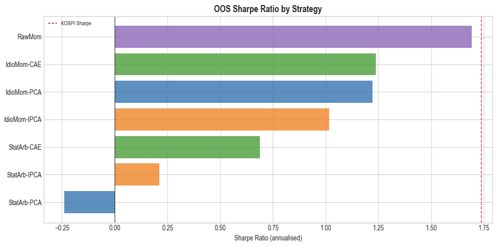
From the summary table and figure 1, I can first compare the factor models within each strategy by their performance, as well as compare the performance across strategy type. Within the statistical arbitrage strategy, and from looking at the sharpe ratio of them, CAE residuals perform much better than IPCA and PCA, and the IPCA residuals performs better than the PCA residuals. This indicates that the higher flexibility a factor model has, the improved tradability residuals have when applied to statistical arbitrage strategy. 

Within the idiosyncratic momentum strategy, CAE residuals still outperform the other two factor models, but a difference from the statistical arbitrage is that PCA performs better than IPCA. Although it varies a little, this still shows how the highest flexibility factor model out of the three, CAE’s residuals perform the best within the strategy with the highest sharpe ratio. 

However, the biggest and clearest overall result is the difference between the two strategy families. The momentum strategies produced much higher annual returns, higher sharpe ratios, and overall better results. From all trading strategies, raw momentum was the most effective strategy in our sample too. 

IV. Discussion

The results indicate that, among the three factor models, the CAE produced the most effective residuals for both the statistical arbitrage and idiosyncratic momentum strategies. This supports the idea that more flexible factor models can generate more tradable residuals. PCA is transparent and stable, but its factor loadings are fixed over time, making it relatively restrictive. IPCA improves on this by allowing factor loadings to vary linearly with stock characteristics. While both PCA and IPCA remain linear models, CAE further allows nonlinear relationships between stock characteristics and factor loadings. The stronger performance of CAE residuals across both trading strategies suggests that this additional flexibility enables the model to better isolate stock-specific return components.

However, the results also show that the choice of trading strategy is just as important as the flexibility of the factor model. Although CAE produced the best-performing residuals among the factor models, the raw momentum strategy outperformed all residual-based strategies, suggesting that simple momentum signals were more effective than residual-based alternatives in the KOSPI market during the sample period. Furthermore, after raw momentum, all three idiosyncratic momentum strategies outperformed the statistical arbitrage strategies.

This drastic difference in performance between momentum strateigies and statistical arbitrage strategies could be explained by the estimated OU parameters. The parameter estimates from the methodology section has revealed that the daily residuals do not follow an OU process. Therefore, the statistical arbitrage strategy, relying heavily on mean reversion and OU derived signals, underperformed relative to momentum strategies. Furthermore, the breakdown of the OU process and the superior performance of momentum strategies suggest that  daily KOSPI residuals in this study’s sample are more effective for capturing persistent stock-specific trends than for exploiting short-term mean reversion. Therefore, while increasing factor model flexibility could improve the quality of the residuals, the profitability of residual-based trading also depends on whether the trading strategy is consistent with the underlying behavior of those residuals.

However, there are several limitations to be considered importantly in this study. First, the stock universe of the data is small and the sample period is relatively short compared with larger asset-pricing studies. This makes the results sensitive to the particular market period and to the stocks in the analysis, which could not make the same result when performed to a larger data set. Second, the data is from Yahoo Finance, which may contain missing values and data quality problems. Third, the back tests in this study do not fully include transaction costs, bid-ask spreads, liquidity constraints, and more. Especially in trading performance studies where small implementation details can strongly affect returns and the results, this must go through consideration. Lastly, Survivorship bias is another important limitation. The sample in this study is built from current large KOSPI stocks that have enough data during the study window, meaning that firms that have disappeared and merged are not fully represented. This can make performance appear better than it would be in reality since only the surviving firms remain in the dataset. In order to eliminate survivorship bias, a stronger design of data to include firms that were in the KOSPI universe at each point in time even if they later disappeared could be used.

Acknowledgment

I would like to express my gratitude to Prof. Panos Parpas at the Department of Computing at Imperial College London for his mentorship and guidance on financial modeling and mathematics studies.

References

1. Kelly, B. T., & Xiu, D. (2021). Factor models, machine learning, and asset pricing. SSRN Electronic Journal. https://doi.org/10.2139/ssrn.3943284
2. Kelly, B. T., Pruitt, S., & Su, Y. (2017). Instrumented Principal Component Analysis. SSRN Electronic Journal. https://doi.org/10.2139/ssrn.2983919
3. Gu, S., Kelly, B. T., & Xiu, D. (2019). Autoencoder Asset Pricing Models. SSRN Electronic Journal. https://doi.org/10.2139/ssrn.3335536
4. Kim, E., Cho, T., Koo, B., & Kang, H.-G. (2023). Conditional autoencoder asset pricing models for the Korean stock market. PLOS ONE, 18(7), e0281783. https://doi.org/10.1371/journal.pone.0281783
5. Ryou, H.-Y., Kim, E., & Kang, H.-G. (2025). Application of Instrumented Principal Component Analysis in Korean Stock Market. Industrial Engineering & Management Systems, 24(4), 571–585. https://doi.org/10.7232/iems.2025.24.4.571
6. Avellaneda, M., & Lee, J.-H. (2008). Statistical Arbitrage in the U.S. Equities Market. SSRN Electronic Journal. https://doi.org/10.2139/ssrn.1153505
7. Akiba, T., Sano, S., Yanase, T., Ohta, T., & Koyama, M. (2019). Optuna: A Next-generation Hyperparameter Optimization Framework. https://arxiv.org/pdf/1907.10902
8. Papanicolaou, G., & Yeo, J. (2016). Risk Control of Mean-Reversion Time in Statistical Arbitrage. SSRN Electronic Journal. https://doi.org/10.2139/ssrn.2868525
9. Blitz, D., Huij, J., & Martens, M. (2009). Residual Momentum. SSRN Electronic Journal. https://doi.org/10.2139/ssrn.2319861

---