Redlining: Quantifying the Economic History of the San Francisco Bay Area

Introduction

“87% of neighborhoods in San Francisco undergoing gentrification were once redlined as hazardous” (“From Redlining to Gentrification: The Policy of the Past that Affects Health Outcomes Today”). Redlining was a discriminatory practice in which banks and government agencies denied services such as insurance and mortgages to residents of neighborhoods with large African American and other minority populations. Over time, this practice caused significant disinvestment and economic deterioration of neighborhoods it affected, leaving many people in a fixed place of poverty that prevented upward socioeconomic mobility.

Established in 1933 as a part of Franklin Delano Roosevelt’s “New Deal” program to lift the country out of economic depression, the Home Owners’ Loan Corporation (HOLC) provided mortgage relief to homeowners at risk of losing their homes through foreclosure, in order to stabilize the housing market. As a part of this process, the HOLC created numerous residential security maps, grading different neighborhoods A-D (A being a highly secure and desirable neighborhood & D being a hazardous neighborhood) in about 200 different U.S. cities. Though aiming to create stability in the housing market, these letter grades were primarily based upon the socioeconomic, racial, and ethnic makeup of the neighborhoods’ residents, which facilitated the development of discrimination in the U.S. housing market. With the Johnson administration’s passage of the Fair Housing Act in 1968, any means of housing discrimination on the basis of race, sex, familial status, nationality, and disability were prohibited, thereby marking the closure of the HOLC’s rampant redlining practices of the mid-20th century. However, despite the practice’s prohibition, redlining had already caused a large amount of socioeconomic damage on the communities it had impacted, through a ripple effect of discrimination prevalent in many of society’s pillar institutions (ie schooling, employment, healthy food access)

In this paper I aim to answer the following question: What are the long-term economic impacts of 1930s-era HOLC redlining in the San Francisco Bay Area? By focusing on the quantitative relationships between redlining tract coverage and census data of racial demographics, household income, educational access, and employment, this paper aims to quantify the extent of redlining’s association with economic disparity throughout the late 20th and early 21st centuries through distributional impacts, categorical comparisons, and regression analysis.

From conducting distributional, categorical, and regression analyses, there are several patterns that can be concluded about the long-term economic impacts of New Deal-era HOLC redlining in the Bay Area. Firstly, the distributions holistically showed minimal change in shape over time indicating that the economic indicators measured stayed consistent over the course of several decades. This consistency goes to show that the economic impacts caused by redlining are solid and aren’t weak enough to change over time. Secondly, the regression analysis showed a negative relationship between income and redlining tract coverage with an increasing slope magnitude over time and a statistically significant relationship between the two variables indicated by the very low p-values.  

Section 1: Distributional Impacts

To examine the persistent long-term economic impacts of redlining across different HOLC-graded neighborhoods (graded on desirability), I first generated histograms of median household income (1980-2000), unemployment (1980-2000), and white-occupied housing (1980-2020) across HOLC grades A-D, which reveal several long term distributional economic trends.

Histograms were chosen because they allow one to see the persistence or change of these economic patterns over time by noticing a persistence of change in the spread and shape of the census data across HOLC grades. The incorporation of histogram series by time period with the four different grades per serie allows one to see variation within each grade and how the socioeconomic indicator of one grade changed over time relative to another. Each histogram plots the relative frequency of a given census variable across HOLC tracts A-D as defined by the 1930s HOLC redlining maps. By using relative frequency histograms rather than raw count histograms, the distributions are normalized which allows for fair and accurate comparison across grades that have a different number of census tracts. To ensure accurate comparability over time, the relative frequency histogram that plots median household income (1980-200) across HOLC grades A-D were converted from nominal US dollars to real 2020 US dollars using the Bureau of Labor Statistics’ annual average CPI values.

Subsection 1A: Median Household Income

The first socioeconomic indicator is real median household income. This variable measures the typical earning level of all households in a neighborhood, which is a strong indicator of overall economic opportunity in that neighborhood. Because nominal incomes change with inflation, the median household incomes were converted from nominal to real 2020 U.S. dollars using annual average CPI values from the U.S. Bureau of Labor Statistics. 

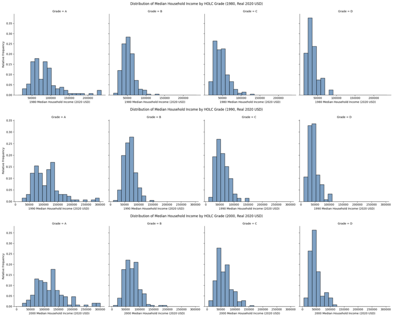
The first observation that can be drawn from Figure 1.1 is that the shape of the distributions of median household income for each HOLC grade remains approximately the same consistently across all three dates of measure. This indicates that aggregate household income for each grade persisted over the period of measure.

The second observation that can be drawn from Figure 1.1 has to do with the differences in intergrade clustering and spread of the data. Grade A’s distribution has a slight right-skew with a moderately-large income range that persists across the three dates of measure. Moving from the Grade A distribution to the Grade D distribution, the data gradually shifts left with each grade closer to D. Grade D’s distribution shows one, a high level of clustering at the left side of the left side of the histogram and two, an income range that is significantly smaller than that of Grade A’s distribution. These two observations continue throughout the three dates of measure.

From these observations, it can be concluded that Grade A Bay Area neighborhoods have a larger range of median household income values with fewer observations of lower median household income values. This conclusion is in accordance with the inference that those in a grade with greater security and desirability tend to have higher job opportunity, educational access, and healthcare access. The subtle right-skew in Grade A’s distribution indicates that a smaller proportion of tracts have exceptionally high incomes which increases the mean and pulls the distribution’s tail rightward. The gradual leftward shift of the distributions from Grade A to Grade D indicates that as the magnitude of risk assessed by the HOLC for the tracts is inversely proportional to the median household income for the tracts. Moving to Grade D, it can be concluded that tracts judged to have lower security and desirability by the HOLC have a smaller range of median household income values and a high proportion of observations of lower median household income. This conclusion is in agreement with the inference that individuals in this grade tend to have lesser job opportunity, lesser educational access, and lesser healthcare access, traits which undermine ability to achieve high household income.

In addition, the moderately-large range of income denoted in Grade A’s distribution hints at a more discrete but key principle of 1930s HOLC redlining: racial prejudice. As observed in Grade D’s distribution, there was a visible clustering of tracts toward the left of the histogram around the lower income values. Intuitively, this logic should apply to Grade A as well but in an opposite fashion: clustering of tracts toward the right of the histogram around the higher income values. However, in Grade A’s distribution there is a significantly-sized range and spread of income, much larger than that of Grade D’s distribution, indicating that Grade A neighborhoods contained households with a variety of median household income values. From this distributional observation, it can be understood that HOLC redlining grading was deeply influenced by racial prejudice, more so than objective economic data for a lot of the time.

Subsection 1B: Unemployment

The second socioeconomic indicator is percent of civilians unemployed (16+). This variable measures the share of the working-class population per grade that are actively seeking employment but cannot find work. Redlined neighborhoods often see disinvestment and lower amounts of socioeconomic mobility so distributional unemployment is a strong indicator of the severity of redlining experienced by grade.

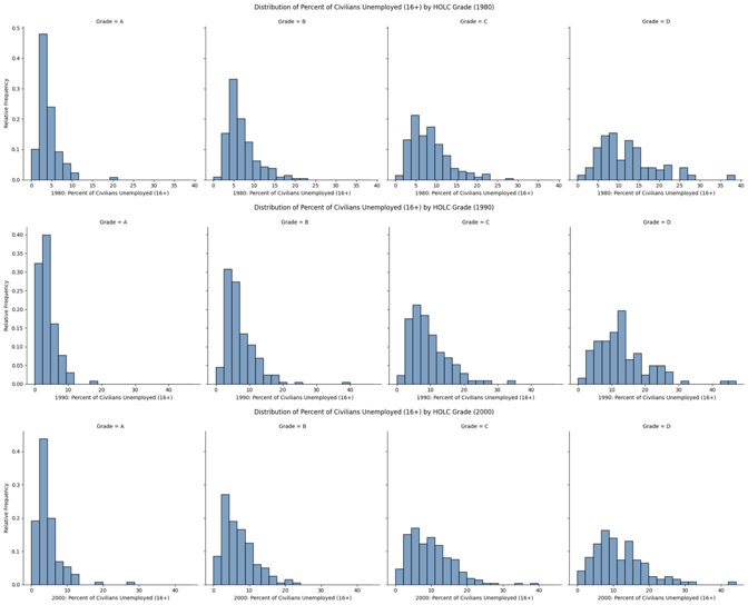
Similar to the distribution of median household income across HOLC grades, the first observation drawn from Figure 1.2 is that consistently across all three dates of measure, the shape of the distribution for each respective HOLC grade remains approximately the same, with only a few minor shifts, which indicates that unemployment shares for each grade persisted over time. This persistence in unemployment suggests that the socioeconomic division caused by 1930s HOLC redlining has stayed relatively intact in the latter half of the 20th century, with census level unemployment shares continuing to mirror structural inequalities imposed by HOLC redlining maps.

The second observation drawn from Figure 1.2 is concerned with the differences in intergrade clustering and spread of the data as well. Generally, these differences are the same as in Figure 1.1 but a mirror flip. Grade A’s distribution shows high left-clustering, a small right-skew, and a very high proportion of observations on that side of the histogram. Moving from the Grade A distribution to the Grade D distribution, the data gradually gains overall spread/range and magnitude of right-skew while also losing peak height. Grade D’s distribution shows a range and median greater than that of Grade A. This pattern of inter-grade shifting from A to D remains approximately the same over the period of measure.

From these observations, it can generally be concluded that the magnitude of risk assessed by the HOLC for the tracts is directly proportional to the percent of civilians (16+) unemployed for the tracts. The association between these two variables is consistent with the inference that redlined neighborhoods tend to have lower economic opportunity, in this case job access, resulting in a higher unemployment rate in these tracts. While the median percent of civilians (16+) unemployed increases moving from Grade A to Grade D, the magnitude of right skew also increases which means that there is a higher degree of variability in tracts deemed less secure and desirable by the HOLC. Economically, this increase in variability in percent of civilians (16+) unemployed from Grade A to Grade D means that the magnitude of risk assessed by the HOLC for the tracts is associated with a higher degree of economic volatility in the tracts. These tracts that have experienced a high amount of redlining have also seen uneven patterns of disinvestment, reinvestment, demographic/population change, gentrification, industrial restructuring, factors which are greatly responsible for a high variation in unemployment in these tracts. In addition to an increase in magnitude of right skew from Grade A to Grade D, a decrease in peak height is also observed. This means the magnitude of risk assessed by the HOLC for the tracts is inversely proportional to the proportion of observations made. Similar to an increase in spread, a decrease in peak height also denotes a proportional relationship between degree of redlining and degree of economic volatility observed. From a statistical standpoint, the decrease in peak height, or flattening, of the distribution means that a fewer proportion of tracts share a common unemployment rate for civilians (16+). This flattening represents a growing internal heterogeneity suggesting that redlining produced a fragmented and nonuniform economic landscape in the areas it greatly impacted.

Subsection 1.C: White Share

The third socioeconomic indicator is percent of white-occupied houses. This variable measures a specific racial composition of occupied housing units. Historically, redlined neighborhoods in the mid 20th century saw a large amount of urban flight in which primarily caucasian residents departed urban areas for suburban neighborhoods. As a result of this exodus, over time, redlined neighborhoods saw a change in white residents so by measuring this variable, we will see how the magnitude and direction of this change across grades and the fluctuations in change over time. 

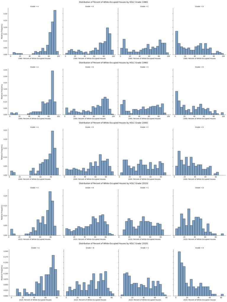
Similar to the previous two distributions, the first observation that can be drawn from Figure 1.3 is that across the five dates of measure, the shape of the distribution for HOLC grades A, B, and C remain approximately the same, with only a few minor shifts. This indicates that for these grades, the distribution of percent of white occupied homes persisted over the course of 4 decades. Likewise to the other socioeconomic indicators measured in Figures 1.1 and 1.2 respectively, the persistence of shares of white occupied homes suggests that the census-level outcomes of the racial bias  ingrained into HOLC redlining maps has seen very minimal change in the highly to moderately secure and desirable tracts (A-C), indicating that housing segregation on the basis of race has persisted over time in the Bay Area.

The second set of observations that can be drawn from Figure 1.3 concerns the shape of each grade’s distribution over the period of measure: what the shape means and for Grade D, what a shift in the distribution’s shape means. Firstly, moving left to right from Grade A to Grade D, there is a gradual flattening of the distribution, most significantly moving from Grade A to Grade B, and there is a shift from a right-skew to a left-skew. Moving vertically down the figure from 1980 to 2020, the distributions of Grades B, C, and D see a subtle and gradual increase in aggregate peak height over time. In Grade D, there is a sharp increase in proportion of observations over time at the 7-20% range of the 2020 distribution.

From these observations, it can be concluded that magnitude of risk assessed by the HOLC for the tracts is inversely proportional to the percent of white-occupied houses for the tracts over time. As the HOLC grade declines in security and desirability, the distribution becomes increasingly concentrated toward lower percentage values of white-occupied houses. This inverse association, shown by the shift of a right-skew to a left-skew from Grade A to Grade D in each date of measure, confirms our understanding of HOLC redlining having a basis of racial prejudice, as lower-tier grades and areas with higher levels of redlining tend to have a greater minority demographic and a lower majority, in this case caucasian, demographic. The flattening of the distributions in the earlier dates of measure (1980 and 1990 primarily) indicate an increase in demographic variability as tracts become more “hazardous.” While secure and desirable areas remain racially homogenous with a high proportion of caucasians, areas with lower security and desirability are more racially heterogenous reflecting both racial segregation’s influence in HOLC redlining as well as subsequent population shifts driven by disinvestment and suburbanization. The increase in overall peak height for Grades B, C, and D but retainment of a roughly flat shape relative to Grade A’s distribution indicate that there is a greater amount of census data concerning white-occupied housing moving forward in time, but the demographic trends revealed by this data remain persistent as mentioned in detail above. The sharp increase in peak height in 2020 at the 7-20% range of the Grade D histogram indicates that there is a significantly higher proportion of observations concentrated around the lower percent of white-occupied houses in recent times, a trend that can be explained by “white-flight” and suburbanization. This migratory occurrence is defined as the migration of primarily caucasian residents from urban to suburban areas, which results in the economic degradation of urban areas through decreased funding and overall maintenance.

Section 2: Categorical / Group-Level Comparisons

To further explore the economic impacts of 1930s HOLC redlining in the Bay Area, I used categorical plots to visualize redlining’s impact through median household income and educational attainment across HOLC grades A-D.

Definitionally, a categorical plot allows for comparison of a single numerical variable across four levels of categorical variables, in this case, each level corresponding to a HOLC grade A-D. The important distinction that needs to be made in order to understand what the differences are in the displaying of categorical variables (HOLC grades) is the difference in interpretation over time for the histograms vs. the categorical plots. The histogram focuses on distributional change within a singular HOLC grade over time, which provides insight into intra-grade socioeconomic change over the period of measure. On the other hand, the categorical plot focuses on the change in inter-grade variation over time for a given socioeconomic indicator.  Due to this difference, I chose to incorporate categorical plots to supplement the distributions in order to visualize comparative disparities between HOLC grades.

Furthermore, in connecting the two models, a single bar within a categorical plot can be interpreted like a distribution for the HOLC grade that the bar represents, through the spread of data points within the bar.

Subsection 2A: Median Household Income

The first socioeconomic indicator to be analyzed categorically is median household income (real 2020 USD) across HOLC grades A-D. In the figure that assesses this variable, there are three categorical plots, one plot for each period of measure, 1980, 1990, and 2000 respectively.

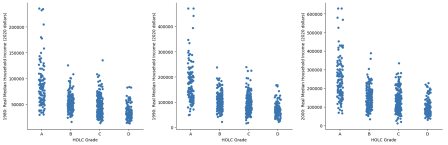
The first observation that can be drawn from Figure 2.1 is the clear downward trend from Grade A to D that is consistent across all three dates of measure, with Grade A having the highest peak and Grade D having the lowest peak. The second observation that can be drawn from Figure 2.1 concerns intra-grade variability indicated by the distribution of data points within each HOLC Grade’s bar. Consistently across all three dates of measure, Grade A tracts show the greatest intra-grade variability, indicated by a greater spread of data points within the bar. As the HOLC grade declines however, there is a decrease in intra-grade variability, indicated by the increasing clustering of data points within each bar. The third observation that can be drawn from Figure 2.1 is an increase in the peak height for each HOLC Grade’s bar over time, while the vertical separation between each bar remains approximately equivalent over time. 

From the first observation, it can be roughly concluded that magnitude of risk and insecurity determined by the HOLC and the median household income are inversely proportional for the tracts. This observation is consistent with the basis of redlining, in which redlined neighborhoods saw high levels of disinvestment and economic deterioration, preventing upward socioeconomic mobility for residents of these tracts, therefore explaining why residents of redlined tracts tended to have lower median incomes than those of non-redlined tracts. From the second observation concerning intra-grade variability, the higher levels of variability in tracts deemed less risky and more secure by the HOLC indicate that in these tracts, there is a greater degree of economic opportunity and mobility, providing an explanation for a wider spread in Grade A and a tighter clustering in lower grades, where many residents of redlined tracts are stuck in a lower socioeconomic position and unable to advance upwards. From the third observation concerning the increase in relative heights of each HOLC Grade’s bar over time, we can conclude that across all tracts, redlined or not, general development over the period of measure through technological innovation and globalization promoted the median household incomes for each HOLC Grade. Despite this overall increase, the vertical separation for each catplot between each HOLC Grade remains approximately equivalent suggesting that relative disparities between grades persisted despite overall income growth over the period of measure.

Subsection 2B: Educational Attainment

The second socioeconomic indicator to be analyzed categorically is educational attainment across HOLC grades A-D. This variable will be measured by the percent of adults 25 and older with 4 or more years of college education. In the figure below, there are three categorical plots, one plot for each period of measure, 1980, 1990, and 2000 respectively.

The first observation that can be drawn from Figure 2.2 is the clear downward trend from Grade A to Grade D across all three dates of measure, with Grade A having the highest peak and Grade A having the lowest peak. The second observation that can be drawn is the gradual upward shift in each grade over time, shown by the increasing peak height for each HOLC Grade’s bar. In connecting these two observations, we see that the difference in peak heights between the HOLC Grades decreases over the period of measure, with the bars for Grades B-D increasing by a greater amount than the bar for Grade A, revealing a flattening of the downward trend from Grade A to D.

From the first observation, it can be concluded that magnitude of risk and insecurity determined by the HOLC is inversely proportional to the percent of adults 25 years of age and older with 4 or more years of college education for the tracts. This conclusion aligns with the economics of redlining in which neighborhoods that experienced the negative implications of the practice saw less economic opportunity as well as overall disinvestment in their communities. Tracking back to Figure 2.1, we see that neighborhoods in lower tier HOLC grades have generally a lower aggregate median household income. Due to the aggregate financial status of these neighborhoods, we can infer that one of the reasons that households in redlined neighborhoods saw lower degrees of educational attainment was they comprehensively had less disposable income to spend on privileges like textbooks, tutoring services, or in this case, a college education.

From the second observation, it can be concluded that the moderate to lower tier grades saw upward educational mobility over the period of measure. This pattern can be primarily attributed to neighborhood redevelopment and gentrification throughout the Bay Area, particularly in tracts close in proximity to university centers, like UC Berkeley, or booming industries that have attracted more college-educated residents in search of work on a domestic and international level, like Silicon Valley and the South Bay. Coinciding with these inferences, the Bay Area saw several urban redevelopment projects in parts of Oakland, Emeryville, and San Francisco’s Mission District in which communities experienced infrastructural improvement in housing and schools. In a research report titled Engaging Schools in Urban Revitalization: The Y-PLAN (Youth – Plan, Learn, Act, Now!), authors Deborah L. McKoy and Jeffrey M. Vincent define the Y-PLAN initiative in the context of the urban Bay Area: 

“West Oakland, California, is an industrial area suffering the abandonment and blight common to other neighborhoods after the loss of manufacturing employers, a process that began in the 1950s…Stepping into this environment in 2000 was the Y-PLAN (Youth—Plan, Learn, Act, Now!), a model for youth civic engagement in city planning that uses urban space slated for redevelopment as a catalyst for community revitalization and education reform. Sponsored by the Center for Cities & Schools at the University of California (UC), Berkeley, Y-PLAN facilitates positive community outcomes by partnering graduate student “mentors,” local high school students, government agencies, private interests, and other community parties to work on a real-world planning issue. The Y-PLAN is both a pedagogical tool and a planning studio that addresses specific issues in local communities” (McKoy & Vincent, 2007, p. 1).

Due to the implementation of programs such as the Y-PLAN that educationally mobilized the Bay Area’s youth in impoverished areas, many of these neighborhood areas saw educational improvement reflected by the increasing peak heights for tracts in HOLC Grades B-D in the categorical plot. As a result of the flattening of the downward trend, it can be concluded that the educational disparities within the Bay Area were ameliorated over the period of measure, in part due to youth initiatives and other programs seeking educational improvement.

Section 3: Regression Analysis of Raw Median Household Income

To determine the impact of redlining tract coverage on median household income, I also conducted ordinary least squares (OLS) linear regressions for both the raw and logarithm of median household income as a function of redlining tract coverage from a 1930s HOLC map. While the histograms and catplots provide distributional insight and categorical comparison, respectively, into disparities across HOLC grades, the regression allows for high quantitative precision in determining the extent to which redlining coverage can accurately predict income for a Bay Area neighborhood. More specifically, the categorical plots allowed us to see a general slope trend based on the peaks of each bar, but the regression expands upon this observation by making it more specific numerically.

Because nominal incomes change with inflation, the median household incomes were converted from nominal to real 2020 U.S. dollars using annual average CPI values from the U.S. Bureau of Labor Statistics. The purpose of conducting a log-transformed regression was to linearize the relationship and allow for the slope coefficient to be interpreted as a percent change in income for a one-unit increase in tract coverage.

The two key regression outputs that will be analyzed in this section are slope coefficient and p-values, which together, can assess the magnitude and certainty, respectively, of the relationship between redlining tract coverage and median household income over time. For the raw income model, the slope coefficient is interpreted as the predicted change in real median household income by the OLS regression line per one-unit (or 100%) increase in redlining tract coverage. For the log-transformed income model, the slope coefficient is interpreted as the predicted percent change in real median household income by the OLS regression line per 1.0 (or 100%) increase in redlining tract coverage. Given that the distribution of income is skewed, taking the logarithm of income compresses high-income and low-income outliers, which creates a more symmetric and homoscedastic residual distribution. The patterns observed in the logarithm-transformed regression are largely identical to those observed in the untransformed regression, so I decided to include logarithm-transformed regression analysis in the first appendix of the paper. The p-values for each model (raw income and log-transformed income) represent the probability of observing each respective slope by random chance. A low p-value (less than the alpha level of 5%) indicates that the observed relationship is unlikely due to random chance.

Several neighborhood wealth-related trends can be concluded from OLS regression analysis of raw and log-transformed real median household income (2020 dollars) as a function of redlining tract coverage from 1980-2000. While quantitative, these patterns share similarities with the distributional trends derived from the histograms showing real median household income (2020 dollars) across HOLC grades A-D described in detail earlier in the paper.

Here, our parameter beta represents the true slope of the population regression line relating the explanatory and response variables of redlining tract coverage and raw income respectively. The null hypothesis is that beta is equal to zero and the alternative hypothesis is that beta is less than zero.

	1980	1990	2000
Coefficient	-15205.29	-29742.12	-46819.90
P-Value	1.8530e-06	7.8373e-06	1.9035e-06

Figure 3.1 Raw Income as a function of Redlining Tract Coverage

Figure 3.1 confirms a negative association between income and redlining tract coverage based on the slope coefficients. Firstly, the slope coefficient for the 1980 OLS regression is -15,205.29. This means that for each additional one-unit (or 100%) increase in redlining tract coverage, the OLS regression line predicts about a $15,205.29 decrease in real median household income (2020 dollars) in 1980. Secondly, the slope coefficient for the 1990 OLS regression is -29,742.12. This means that for each additional one-unit (or 100%) increase in redlining tract coverage, the OLS regression line predicts about a $29,742.12 decrease in real median household income (2020 dollars) in 1990. Thirdly, the slope coefficient for the 2000 OLS regression is -46,819.90. This means that for each additional one-unit (or 100%) increase in redlining tract coverage, the OLS regression line predicts about a $46,819.90 decrease in real median household income (2020 dollars) in 2000.

While I noted that the association between income and redlining tract coverage remains negative, from the slope coefficients in Figure 3.1, it can also be observed that the magnitude of the decrease in income increases with each subsequent date of measure. From a graphical standpoint, this can be understood as an initially negative regression line that gets steeper and steeper in the negative direction over time. So what does this mean in the context of redlining? From this observation, it can be concluded that the negative impact of redlining coverage on household income worsens overtime, as the same increase in coverage is met with a greater magnitude of decrease in income over the period of measure. This trend can be best explained by the extensive impact of disinvestment in higher redlined areas. Following the HOLC’s classification of neighborhoods as “hazardous” via their redlining maps, banks and financial institutions chose not to lend money to businesses and individuals, insure mortgages, or fund development in these areas due to the high-risk attributed to these areas by the HOLC. As a result of this lack of financial and infrastructural support from banking institutions, these areas deteriorated over time through an aggregate decrease in property values as well as less socioeconomic mobility and in this case, access to high-paying jobs. Due to the extensive decline of the economic makeup of these areas caused by disinvestment, it makes sense why the slope coefficient of the income vs. redlining tract coverage regression decrease over time.

Figure 3.1 also displays very low p-values that all fall significantly below the general alpha level of 5%. Therefore, we can ascertain a relationship between redlining tract coverage and income. Firstly, the p-value for the 1980 OLS regression with raw income as the dependent variable is  . Assuming that there’s no association between redlining tract coverage and real median household income in 1980, the probability of obtaining a sample of this size and observing a negative relationship between redlining tract coverage and real median household income (2020 dollars) as or more extreme than a magnitude of approximately $15,205.29 per percentage point of redlining tract coverage by random chance is less than approximately   (rounded 0.0002%). Therefore, the OLS regression model provides significant statistical evidence that tracts with higher redlining coverage are associated with lower real median household income in 1980 for this sample. Secondly, the p-value for the 1990 OLS regression with raw income as the dependent variable is  . Assuming that there’s no association between redlining tract coverage and real median household income in 1990, the probability of obtaining a sample of this size and observing a negative relationship between redlining tract coverage and real median household income (2020 dollars) as or more extreme than a magnitude of approximately $29,742.12 per percentage point of redlining tract coverage by random chance is less than   (rounded 0.0008%). Therefore, the OLS regression model provides significant statistical evidence that tracts with higher redlining coverage are associated with lower real median household income 1990. Thirdly, the p-value for the 2000 OLS regression with raw income as the dependent variable is  . Assuming that there’s no association between redlining tract coverage and real median household income in 2000, the probability of obtaining a sample of this size and observing a negative relationship between redlining tract coverage and real median household income (2020 dollars) as or more extreme than a magnitude of approximately $46,819.90 per percentage point of redlining tract coverage by random chance is less than   (rounded 0.0002%). Therefore, the OLS regression model provides significant statistical evidence that tracts with higher redlining coverage are associated with lower real median household income 2000.

The consistently low p-values across all three dates of measure (less than the alpha level of 5%) confirms the high statistical strength between redlining tract coverage as an independent variable and median household income as a dependent variable. Furthermore, this aspect of the regression corroborates the trends observed from the slope coefficients of the decreasing negative association between these two variables, indicating that it is extremely unlikely this relationship occurred by random chance.

Conclusion

From distributional impacts, to categorical plots, to regression analysis, we can conclude several long term economic impacts that vary by extent to which a given census tract was redlined and how it changed over time. With the histograms, we saw that a lot of the economic patterns surrounding income and unemployment maintained shape for a given grade distribution over time indicating that a lot of the economic impacts stayed stagnant over the course of a few decades. With the regression analysis, we saw that the magnitude of negative slope for raw income as a function of redlining tract coverage greatly decreased in the 20 year period from around $30,000 to $42,000 in 1980 and 2000 respectively. With the log transformed regression, the slope coefficients were approximately equivalent for each year indicating that income dropped by the same percentage each year which shows relative stability in the influence of redlining, not due to external factors.

Looking forward, I would love to dive deeper into how gentrification interacts with these socioeconomic patterns of redlining. By definition, gentrification is the process in which a poorer area is infrastructurally improved as a result of a wealthier demographic of people moving in. This economic improvement is seen over time through improved housing, healthcare, and new business. By exploring gentrification in the context of redlining, I would ask whether modern reinvestment in previously redlined areas resulted in economic growth, ameliorating the negative effects of 1930s-era HOLC redlining.

While in this paper, I primarily studied solely socioeconomic indicators measuring the effects of redlining (unemployment, income, racial demographics, etc.), I would be curious to explore more health-related effects of this same era of redlining. By conducting research on food deserts, urban areas with limited access to good-quality fresh food, through measuring, for example, the number of fast food restaurants in a given census tract as well as illnesses through measuring, for example, the number of diabetes occurrences or hospital visits in a given census tract, I would bring in a new dimension of human health and biology in association with the redlining I explored in this paper. 

Bibliography

De los Santos, H., Jiang, K., Bernardi, J., & Okechukwu, C. (2021, May 26). From redlining to gentrification: The policy of the past that affects health outcomes today. Harvard Medical Journal. Retrieved October 28, 2025, from https://info.primarycare.hms.harvard.edu/perspectives/articles/redlining-gentrification-health-outcomes

Jonathan Schroeder, David Van Riper, Steven Manson, Katherine Knowles, Tracy Kugler, Finn Roberts, and Steven Ruggles. IPUMS National Historical Geographic Information System: Version 20.0 [dataset]. Minneapolis, MN: IPUMS. 2025. http://doi.org/10.18128/D050.V20.0

McKoy, D. L., & Vincent, J. M. (2007, June). Engaging schools in urban revitalization: The y-PLAN. Association of Collegiate Schools of Planning. https://doi.org/10.1177/0739456×06298817

Nelson, R. K., Winling, L, et al. (2023). Mapping Inequality: Redlining in New Deal America. Digital Scholarship Lab. https://dsl.richmond.edu/panorama/redlininghttps://dsl.richmond.edu/panorama/redlining.

Appendix A: Regression Analysis of the Logarithm of Median Household Income

While the raw-income regression shows the dollar change in income as a function of redlining tract coverage, by taking the logarithm of income and performing the same regression function, we see the percent change in income as a function of redlining tract coverage for the same three dates of measure. Though not visible from the regression outputs, the log-transformed regression mitigates the effect of outliers and influential points that undermined the strength of the relationship between raw-income and redlining tract coverage, providing us slope coefficients and p-values that are optimal for ensuring an accurate relationship between the two variables.

Here, our parameter beta represents the true slope of the population regression line relating the explanatory and response variables of redlining tract coverage and logarithm of income respectively. The null hypothesis is that beta is equal to zero and the alternative hypothesis is that beta is less than zero.

	1980	1990	2000
Coefficient	-0.30	-0.28	-0.32
P-Value	(8.3706e-09)	(6.0757e-07)	(1.3727e-07)

Figure A1 Logarithm of Income as a function of Redlining Tract Coverage

Similar to the raw income regression, the results of the log-transformed regression shown in Figure A1 confirm a negative association between redlining tract coverage and income as well. The slope coefficient for the 1980 OLS regression is -0.30. This means that for each additional one-unit (or 100%) increase in redlining tract coverage, the OLS regression line predicts about a 30% decrease in real median household income (2020 dollars) in 1980. The slope coefficient for the 1990 OLS regression is -0.28. This means that for each additional one-unit (or 100%) increase in redlining tract coverage, the OLS regression line predicts about a 28% decrease in real median household income (2020 dollars) in 1980. The slope coefficient for the 2000 OLS regression is -0.32. This means that for each additional one-unit (or 100%) increase in redlining tract coverage, the OLS regression line predicts about a 32% decrease in real median household income (2020 dollars) in 1980.

Similar to the raw income regression, the results of the log-transformed income regression evidenced in Figure A1 show very low p-values. Therefore, we can ascertain a relationship between redlining tract coverage and income. The p-value for the 1980 OLS regression is  . Assuming that there is no relationship between redlining tract coverage and the logarithm of real median household income in 1980, the probability of obtaining a sample of this size and observing a linear relationship between redlining tract coverage and the logarithm of real median household income (2020 dollars) with a slope coefficient of -0.30 or less by random chance alone is less than  %. Therefore, the OLS regression model provides significant statistical evidence that tracts with higher redlining coverage are associated with lower proportional levels of real median household income in 1980. The p-value for the 1990 OLS regression is  . Assuming that there is no relationship between redlining tract coverage and the logarithm of real median household income in 1990, the probability of obtaining a sample of this size and observing a linear relationship between redlining tract coverage and the logarithm of real median household income (2020 dollars) with a slope coefficient of -0.28 or less by random chance alone is less than  . Therefore, the OLS regression model provides significant statistical evidence that tracts with higher redlining coverage are associated with lower proportional levels of real median household income in 1990. Lastly, the p-value for the 2000 OLS regression is  . Assuming that there is no relationship between redlining tract coverage and the logarithm of real median household income in 2000, the probability of obtaining a sample of this size and observing a linear relationship between redlining tract coverage and the logarithm of real median household income (2020 dollars) with a slope coefficient of -0.32 or less by random chance alone is less than  . Therefore, the OLS regression model provides significant statistical evidence that tracts with higher redlining coverage are associated with lower proportional levels of real median household income in 2000.

For the most part, these two outputs of the regression reveal largely similar or identical patterns as the raw-income regression. Firstly, the slope coefficients reveal a negative relationship between redlining tract coverage and median household income that steepens over time. This steepening means that the percent decrease in median household income per 100% increase in redlining tract coverage increases with each subsequent date of measure.

Again, the p-values for this regression are far below the alpha level of 5% meaning that a relationship between redlining tract coverage and the logarithm of income is statistically significant across all three dates of measure, and not due to random chance.

---