Distributed Sensor Networks: An Analysis of Connectivity and Resilience in Environmental Contexts

Abstract

Distributed sensor networks are exceptional tools in the realm of data collection and environmental monitoring. They have and will continue to see large-scale application in geographical environments, in which they are regularly exposed to obstacles that impede communications as well as node failures that damage network integrity. This paper presents findings that can be used to help network designers utilize optimal parameters for their desired levels of network connectivity and resilience. This paper focuses on the K-Out Graph and the K-Random-Intersection Graph (KRIG) models, each employing a distinct key selection protocol. Using Python and NetworkX, the two models were tested under various conditions designed to mimic real-world network stresses and limitations.  For certain tests, the graphs were also intersected with the Random Geometric Graph (RGG) model to simulate real-world limitations in the form of maximum sensor transmission range. Two metrics were used to measure network resilience, in addition to probability of connectivity. The results were graphed, and it was found that the K-Out model demonstrated higher levels of resilience against node failures, while the KRIG model displayed a higher probability of network connectivity. 

I. Introduction and Variables

The following variables are referred to throughout this paper:

N = Size of network, in number of nodes
m = Size of key pool in KRIG model
S = Choice set for each node (from pool of nodes in K-Out model, and from key ring in KRIG model
K = Size of choice set for each node
r = Transmission radius, or the maximum distance that can separate two connected nodes in RGG model

Distributed sensor networks are groups of wirelessly connected sensors that collect data from their surrounding area. Often, they consist of hundreds to thousands of low-cost units with constrained power capacity, short transmission ranges, and limited computational and storage capabilities. The collected data is relayed between the sensors towards the base station, a more powerful network component that can store and communicate the information to its intended destination. 

Before data collection can begin, sensors must first be distributed across the area of interest. This deployment can happen in numerous ways, such as manual installment and aerial scattering [1]. The former is better suited for smaller networks with a more concentrated group of sensors, whereas a latter is better suited for large-scale networks, especially in remote regions with unfamiliar terrain. 

When deployed over long periods of time, sensor networks can provide comprehensive data reports about their environment, which researchers can conveniently analyze from remote destinations. Coupled with the fact that individual sensors can be customized to collect a wide range of data on physical conditions, such as temperature and humidity [2], this property makes them extremely effective tools in the field of environmental monitoring. In the agricultural industry, for example, sensor networks allow for self regulating greenhouses that promote healthy plant growth and increase agricultural productivity by monitoring and adjusting weather parameters [3]. Another project named SensorScope used sensor networks as a cost-efficient alternative to large sensing stations, and collected data on water quality, evaporation, and mud streams in various locations across Switzerland [4].  

Due to the distinct conditions that they face and the varying purposes for which they are deployed, all sensor networks cannot operate optimally under the same set of parameters. By using simulations to analyze the performance of theoretical networks under various conditions, we can gain valuable insight into how real sensor networks behave when deployed, serving to enhance their performance in the future.

II. Methods

To create these theoretical networks, this paper focuses on the use of K-Out Graph and K-Random-Intersection Graph (KRIG) models. To make this paper’s analysis meaningful, it is crucial to understand how each model functions. First, in either model, nodes are uniformly randomly distributed in a 2-dimensional area. This is akin to real-world deployment in which knowledge of the area is often not known prior to sensor installment, such as in a remote forest. Next, edges are created between the nodes. Depending on the model’s key distribution scheme, the criteria that must be met for the creation of an edge is different. In the K-Out model, each of the N nodes creates a choice set S consisting of K other nodes, which are selected uniformly at random and independently of the other nodes. Then, an undirected edge (can be traversed in both directions) is created between any two nodes N_A and N_B in the network if N_A ϵ S_B, or N_B ϵ S_A, or both. A unique pairwise key is then assigned to both N_A and N_B, allowing them to securely communicate. In the KRIG model, each node creates its choice set S by selecting K items from the shared key pool of m keys uniformly at random and independently of the other nodes. An undirected edge is created between any two nodes N_A and N_B if an item C exists such that C ϵ S_A and C ϵ S_B. The Random Geometric Graph (RGG) model is used in conjunction with the KRIG and K-Out models to simulate limitations on node transmission range. In the RGG model, an edge is created between any two nodes N_A and N_B if the distance that separates them is less than a given radius R.

For both models, testing resiliency involved removing varying numbers of nodes from the network and analyzing the resulting safe graph. However, the process of creating the safe graph was different for each model. In the K-out model, only edges connected to captured nodes were considered compromised. In other words, an edge between V_A and V_B can only be compromised if at least one of V_A or V_B is captured. This is the case because in the K-Out model, V_A and V_B communicate using a unique pairwise key, and that key is not used anywhere else in the network. In the KRIG model, keys are not unique to pairs of connected nodes. Rather, they are sampled from the same key pool by all nodes. This means that an edge between V_A and V_B can be compromised even if neither V_A nor V_B are captured. This happens when the key used to secure communications between V_A and V_B is also held by some node V_K that has been captured.

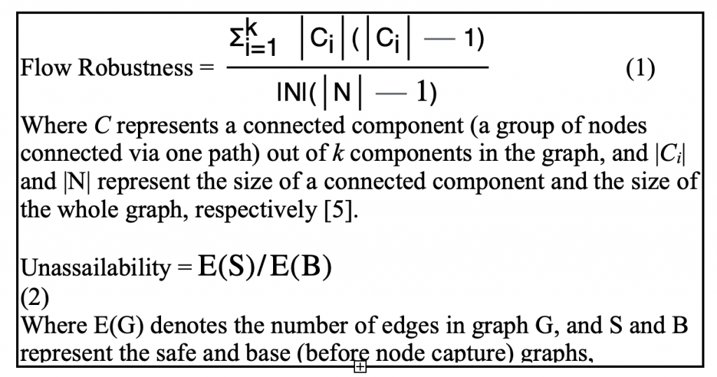
The safe graphs were analyzed using the following metrics:

III. Results and Discussion

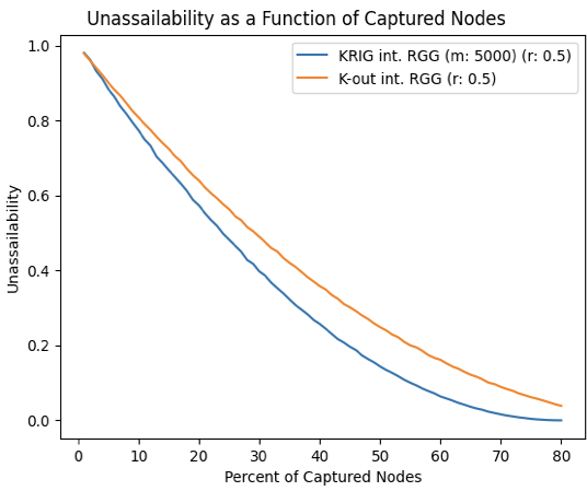
In terms of network resilience, the K-Out model performed noticeably better than the KRIG model (Fig. 1), which can be explained by their key distribution schemes. A captured node in the K-Out model does not have the potential to compromise any nodes other than those it is connected to. This is because the pairwise key distribution ensures that keys are unique to each pair of nodes In the KRIG model, however, a captured node has the potential to compromise multiple other nodes that it shares keys with, as all keys are sampled from the same pool. As a result, the KRIG model is less resilient to random node captures than the K-Out model. 

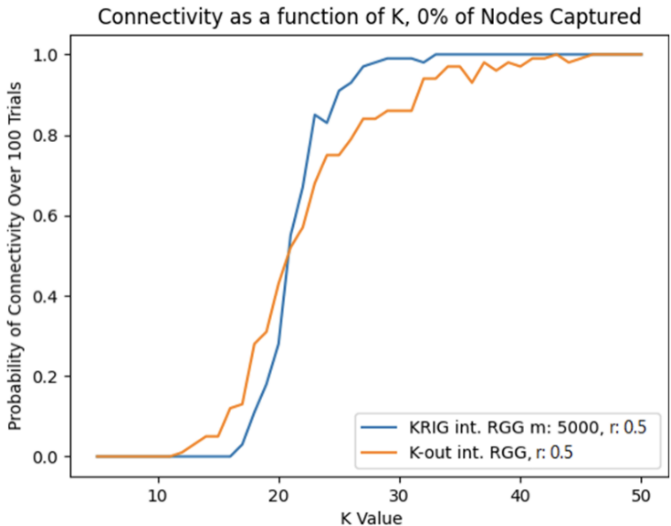
Compared to the K-Out model, the KRIG model displayed significantly higher levels of connectivity at K values past 20, as well much steeper growth as its K value increased (Fig. 2). 

These results demonstrate the inherent trade-off between connectivity and resilience that exists in most current networks [7]. Network designers may use these findings to alter their model and tweak their parameters accordingly. For applications that involve sensor network use in a safe environment, such as greenhouse monitoring, a model that maximizes connectivity is preferred, which in this case is the KRIG model. Using KRIG, 100% network connectivity can be achieved with relatively low K values. In practice, this frees much of the sensors’ bandwidth for other important processes, such as regularly communicating collected data to a web database [8]. 

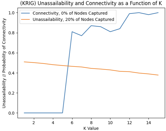
When comparing the unassailability and connectivity of the KRIG model side by side, we see a clear trade-off occurring between them (Fig. 3). This is explained by its key distribution protocol, which leads to more initial connectivity, but decreased resilience as more nodes are captured. This trade-off trend can be utilized to enhance network performance when details regarding the risk that the network faces as well as the duration of network use are available. Higher K values provide higher initial connectivity; therefore, they may be better suited towards short-term uses and/or lower risk areas. Conversely, lower K values provide better resilience against node failure but decreased initial connectivity, making them better suited towards long-term uses and/or higher risk areas.

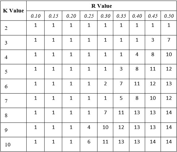
Flow robustness is a measure of the remaining reliable flows in the network, which makes it as strong indicator of how resilient a network is to node capture. In Table 1, K-Out networks with different combinations of K and r parameters were exposed to random node captures, and the smallest integer percentage of captured nodes that caused flow robustness to fall below the threshold of 0.75 was recorded for each combination. As K and r increased, each node had a higher chance of forming an edge with another, either through the additional probability of a shared key or the larger radius that they could be positioned in. This ultimately led to more connected components in the network, and thus more node captures were required to reduce flow robustness below the threshold (Table 1). Due to bandwidth limitations, sensors can face a challenge in the form of short transmission ranges [9]. As illustrated by Table 1, a higher K value can compensate for a lower r value in terms of maintaining flow robustness, therefore sensors with such limitations would likely benefit from utilizing a higher K value, provided they have the necessary memory capabilities to do so. For an existing network, this change would increase the probability that sensors already placed within distance r of one another get assigned a pair-wise key, thereby increasing the total number of connections. 

IV. Conclusion

The properties of the key distribution models analyzed in this paper have the potential to improve sensor networks in various environmental applications such as water quality monitoring, precision agriculture, and natural disaster monitoring [10] [11] [12]. Network designers can utilize the trade-off between initial connectivity and long-term resilience to optimize their networks by adjusting the K value of their sensors depending on the risk level and expected duration of the project. In any network that utilises a pair-wise key distribution scheme, the relationship explored between K and r is useful when combatting sensor limitations. For future research, a comparison between the relatively small-scale networks analyzed in this paper and larger networks made up of thousands of nodes might prove useful; it may be found that network parameters have different impacts on connectivity and resilience depending on the size of the network. In large-scale applications of sensor networks, such as monitoring water quality in oceans, these additional findings will prove useful. Furthermore, testing conditions that mimic real life more closely—such as simulations of 3-D topology in the deployment area—as well as comparisons with other graph models would create a more enhanced view of network behaviour and provide further insight into trade-offs between parameters.

References

[1] Random Key Predistribution Schemes for Sensor Networks. Haowen Chan. (n.d.). Retrieved from https://www.cs.cmu.edu/~haowen/

[2] Ouni, R., & Saleem, K. (2022, July 27). Sustainable Wireless Sensor Network based environmental monitoring. Encyclopedia. Retrieved from https://encyclopedia.pub/entry/25438 

[3] Oo, Z. Z., & Phyu, S. (2021, May 3). Greenhouse Environment Monitoring and controlling system based on IOT Technology. AIP Publishing. Retrieved from https://aip.scitation.org/doi/abs/10.1063/5.0045617 

[4] Barrenetxea, G., Vetterli, M., Schaefer, G., & Ingelrest, F. (2008, May). (PDF) SensorScope: Out-of-the-box environmental monitoring – researchgate. ResearchGate. Retrieved from https://www.researchgate.net/publication/4333845_SensorScope_Out-of-the-Box_Environmental_Monitoring 

[5] Alenazi, M. J. F., & Sterbenz, J. P. G. (2015, October). Evaluation and comparison of several graph robustness metrics to improvenetwork resilience. ResearchGate. Retrieved from https://www.researchgate.net/publication/308604799_Evaluation_and_comparison_of_several_
graph_robustness_metrics_to_improve_network_resilience 

[6] Yagan, O., & Makowski, A. M. (2016, March 11). Wireless sensor networks under the Random Pairwise Key predistribution scheme:  Can resiliency be achieved with small key rings? IEEE Xplore. Retrieved from https://ieeexplore.ieee.org/abstract/document/7431993

[7] Ometov, A., Bezzateev, S., Voloshina, N., Masek, P., & Komarov, M. (2019, December 16). Environmental monitoring with distributed mesh networks: An overview and practical implementation perspective for urban scenario. Sensors (Basel, Switzerland). Retrieved from https://www.ncbi.nlm.nih.gov/pmc/articles/PMC6960639/ 

[8] Račiukaitis, G., Simniškis , R., Šlekas , G., Ragulis, P., Trusovas , R., Ratautas, K., & Duobiene, S. (n.d.). Wireless Sensor Network in Environment Monitoring. Encyclopedia. Retrieved from https://encyclopedia.pub/entry/26027 

[9] Yalavigi, S. Y., Krishnamurthy, D., & NandiniSidnal, D. (2016, July 7). Issues and challenges in Distributed Sensor Networks-A Review. IOSR Journal of Computer Engineering. Retrieved from https://www.academia.edu/26823086/Issues_and_Challenges_in_Distributed_Sensor_Networks_A_Review 

[10] Olatinwo, S. O., & Joubert, T.-H. (2019, March 1). Energy Efficient Solutions in wireless sensor systems for Water Quality Monitoring: A Review. IEEE Xplore. Retrieved from https://ieeexplore.ieee.org/document/8540915 

[11] Jawad, H. M., Nordin, R., Gharghan, S. K., Jawad, A. M., & Ismail, M. (2017, August 3). Energy-efficient wireless sensor networks for Precision Agriculture: A Review. MDPI. Retrieved from https://www.mdpi.com/1424-8220/17/8/1781 

[12] Hart, J. K., & Martinez, K. (2006, July 7). Environmental Sensor Networks: A revolution in the earth system science? Earth-Science Reviews. Retrieved from https://www.sciencedirect.com/science/article/abs/pii/S0012825206000511?via%3Dihub

---