

Author: Nour Saffar Rivas
Mentor: Dr. Ella Atkins
Eton School Mexico
Abstract
This project investigates the design of a simplified Earth-to-Jupiter spacecraft mission using the patched-conic approximation. The mission is modelled using the Sun, Earth, and Jupiter, with all planetary orbits assumed to be circular and coplanar, and a Hohmann transfer orbit is used to model the spacecraft’s heliocentric trajectory. MATLAB is used to perform the numerical calculations and visualize the resulting trajectories. The transfer takes 997.9 days (about 2.73 years), with the departure burn occurring 191.0 days after the initial planetary alignment. Departure from a 5×10⁷ m Earth parking orbit requires Δv = 6,834 m/s, while capture into a circular 2×10⁸ m orbit at Jupiter requires 10,870 m/s, giving a total Δv of 17,704 m/s, of which capture accounts for 61%. Jupiter’s sphere of influence has a radius of 4.82×10¹⁰ m (0.322 AU). A comparison with the Galileo mission, whose capture burn was only about 630 m/s, suggests that the high capture cost in this model comes mainly from the choice of a circular capture orbit.
1 Introduction
Unlike motion around a single body, an interplanetary transfer involves changes between different gravitational regimes, making the direct modeling of a spacecraft’s motion considerably more complex. Mathematical approximations are therefore required to represent these systems while retaining the fundamental relationships that govern orbital motion. The patched-conic approximation provides one of these approaches by treating the spacecraft’s trajectory as a sequence of two-body problems. Within each region of the trajectory, the gravitational influence of one body is assumed to dominate, allowing the spacecraft’s motion to be described using established orbital mechanics. For transfers between approximately circular planetary orbits, a Hohmann transfer provides a particularly simple model of the heliocentric portion of the trajectory. This investigation applies these approximations to an Earth-to-Jupiter transfer. The spacecraft is initially placed in a circular Earth orbit and ultimately enters a circular orbit around Jupiter. MATLAB is used to examine the resulting trajectory and the conditions required for the transfer.
2 Mathematical Background
2.1 Gravitational Parameter and Circular Orbits
A spacecraft traveling through space is constantly affected by the gravitational attraction of nearby celestial bodies. Newton’s law of universal gravitation gives the attractive force between two bodies as
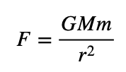
where G is the gravitational constant, M is the mass of the central body, m is the mass of the spacecraft, and r is the distance between their centers of mass (Curtis, 2021). It is standard in orbital mechanics to combine G and M into a single gravitational parameter,
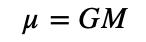
where μ has units of m³ s⁻². Using this parameter, the gravitational force can be expressed as:
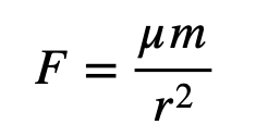
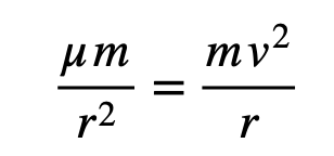
Since μ depends on the central body, the Sun, Earth, and Jupiter each have their own value; this becomes important later, as the model shifts between Earth-centred, Sun-centred, and Jupiter-centred motion. In the case of a circular orbit, gravity supplies the centripetal force needed to keep the spacecraft on its curved path:
After rearranging, the orbital velocity is the following:
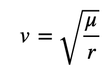
The circular orbital velocity therefore depends only on the distance from the central body and on that body’s gravitational parameter.
2.2 Elliptical Orbits
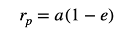
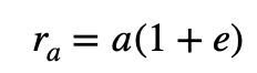
The Earth-to-Jupiter transfer trajectory is not circular but elliptical. An ellipse is described by its semi-major axis a, which represents half of the ellipse’s longest diameter and therefore determines its overall size and its eccentricity e which describes how stretched the ellipse is. In the case of the circle e = 0, while increasing values of e correspond to increasingly elongated ellipses (Atkins, 2019). Along an ellipse, the distance from the central body varies between a closest point, periapsis, and a furthest point, apoapsis. Their distances from the central body are
and
Since these are the two extreme points of the orbit, they can also be used to determine the eccentricity:
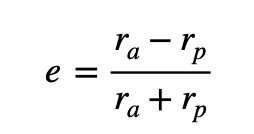
On this paper, Earth’s orbital radius is treated as the periapsis of the heliocentric transfer ellipse, while Jupiter’s is treated as its apoapsis. Consequently, the size and shape of the transfer trajectory are set entirely by the two planets’ orbital radii.
2.3 Vis-Viva Equation
Along an elliptical orbit the spacecraft’s speed is not constant: it moves fastest at periapsis and slowest at apoapsis. This behaviour follows from conservation of specific mechanical energy, ε, the sum of specific kinetic and potential energy, which remains constant everywhere on the orbit:
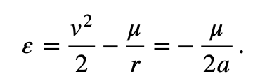
Rearranging for v gives the vis-viva equation (Curtis, 2021):
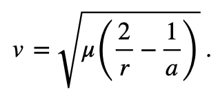
Because a is fixed for a given orbit, this equation can be applied at different points along the same ellipse to determine how the spacecraft’s speed changes with distance r. For the Earth-to-Jupiter transfer, it is used to find the spacecraft’s heliocentric speed at both Earth’s and Jupiter’s orbital radii. These speeds differ from the planets’ own orbital speeds, which is why burns are needed at departure and arrival.
2.4 Hohmann Transfer
A Hohmann transfer connects two circular orbits about a common central body with a single elliptical trajectory tangent to both: periapsis at the inner orbit, apoapsis at the outer one (NASA, 2023). Taking the Sun as the central body, the transfer ellipse spans Earth’s and Jupiter’s heliocentric radii, giving
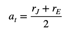
and the eccentricity of this transfer is therefore:
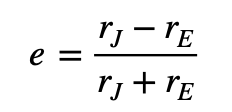
where rE and rJ are the heliocentric orbital radii of Earth and Jupiter. The vis-viva equation then gives the spacecraft’s heliocentric speeds at departure and arrival:
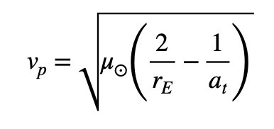
and
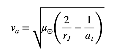
Since the transfer covers exactly half of the ellipse, the transfer time is half the ellipse’s orbital period:
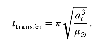
The required velocity changes at departure and arrival, Δv = vfinal − vinitial, sum to the mission’s total delta-v, Δvtotal = Δvdep + Δvarr. Knowing the transfer time alone, however, is not sufficient: Earth and Jupiter continue moving while the spacecraft is in transit, so their motion must also be modeled (Atkins, 2019).
2.5 Planetary Orbital Motion and Launch Geometry
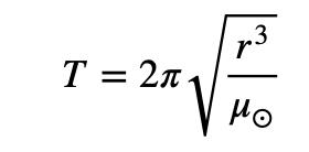
For a circular heliocentric orbit, the period and mean angular velocity or mean motion are:
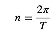
From the period, the mean angular velocity can be found:
Under the assumption of uniform circular motion, the angular position of a planet can therefore be written as
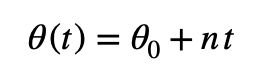
where θ0 is the initial angular position. This allows the prediction of where Earth and Jupiter will be at a particular time. This is key because the spacecraft’s arrival must be synchronized with Jupiter’s position.
2.6 Patched-Conic Approximation
Treating the Sun as the only gravitational influence is reasonable while the spacecraft is far from the planets, but not close to either one. In reality the spacecraft is affected simultaneously by the Sun, Earth, and Jupiter. The patched-conic approximation avoids the resulting many-body problem by dividing the trajectory into regions, each dominated by a single body: an Earth-centred departure, a Sun-centred transfer, and a Jupiter-centred arrival, treated as a sequence of two-body problems and joined at their boundaries (Schaub, n.d.).
2.7 Sphere of Influence
The boundary between regions is approximated by the sphere of influence (SOI), the region around a planet within which its own gravity is treated as dominant, where its approximate radius is
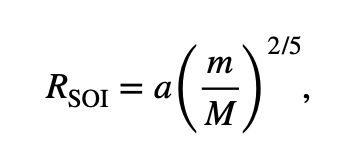
Using gravitational parameters as an equivalent mass ratio, Jupiter’s SOI radius is
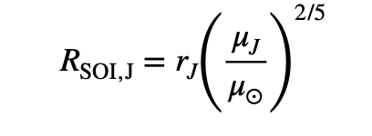
(Lutze, n.d.), giving the model an approximate radius at which the spacecraft’s motion transitions from Sun-centred to Jupiter-centred.
2.8 Hyperbolic Departure and Arrival
Relative to a planet, the spacecraft’s escape or approach trajectory is hyperbolic. Its hyperbolic excess velocity, v∞, is the spacecraft’s velocity relative to the planet once the planet’s gravity becomes negligible. At departure this is the difference between the spacecraft’s heliocentric transfer velocity and Earth’s own orbital velocity,
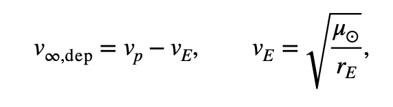
and similarly at arrival,
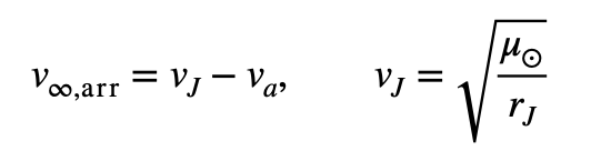
(Atkins, 2021). Closer to the planet, the spacecraft’s speed at periapsis of the hyperbola is
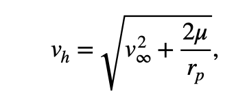
and comparing this to the circular parking-orbit speed, vpark = √(μ/rp), gives the required maneuvre:
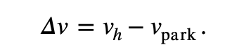
This is applied separately at Earth’s departure and Jupiter’s arrival.
2.9 Hyperbolic Eccentricity and Turn Angle
Eccentricity also describes the shape of a hyperbola, for which e > 1. For the hyperbolic trajectory considered in this investigation, the eccentricity can be determined from the periapsis radius and hyperbolic excess velocity:
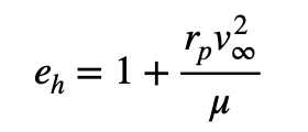
As it passes through the planet’s gravitational field, its velocity changes direction. The amount by which the trajectory is deflected is described by the hyperbolic turn angle:
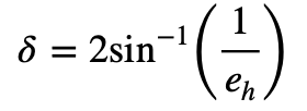
The MATLAB model calculates these quantities for both the Earth departure hyperbola and the Jupiter arrival hyperbola.
2.10 Time of Flight Along the Transfer Orbit
The Hohmann transfer equation gives the total time required to travel from Earth’s orbital radius to Jupiter’s orbital radius. However, the patched-conic model must also determine the time at which the spacecraft reaches the boundary of Jupiter’s sphere of influence. One way of describing the position of a spacecraft on an ellipse is through the eccentric anomaly, E. Unlike the true geometric angle, it makes the relationship between position and time easier to establish. The radial distance from the central body can be written as
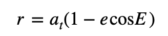
Once the spacecraft’s radial distance is known, this relationship can be used to determine the corresponding eccentric anomaly. The eccentric anomaly is then connected to the mean anomaly, M, through Kepler’s equation:
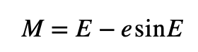
This equation is important because the mean anomaly changes uniformly with time, unlike the spacecraft’s actual angular position along the ellipse. The relationship between mean anomaly and time is
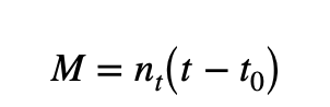
where the mean motion of the transfer ellipse is:
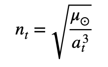
This allows the model to determine the time at which the spacecraft reaches Jupiter’s sphere of influence rather than assuming that the transition occurs at the end of the total Hohmann transfer.
2.11 Hyperbolic Time of Flight
The same idea of relating position to time is required for the Earth-centred hyperbolic departure. Once the spacecraft leaves its circular parking orbit, it follows a hyperbolic trajectory relative to Earth. The model therefore needs to determine how long this phase lasts before the spacecraft approaches its hyperbolic excess velocity. The semi-major axis of a hyperbolic orbit is negative and is given by:
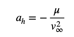
The semi-latus rectum is:
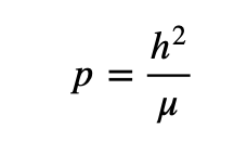
where h is the specific angular momentum. The hyperbolic equivalent of the eccentric anomaly is the hyperbolic anomaly, F. It is related to the hyperbolic mean anomaly Mh by:
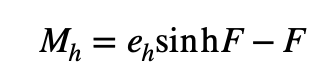
The corresponding hyperbolic mean motion is:
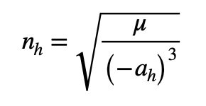
Therefore, the elapsed time can be obtained by:
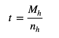
These equations allow the model to connect the spacecraft’s position on its Earth-centred hyperbola with the time elapsed since the departure maneuvre. In this investigation, this is used to determine the time required for the spacecraft’s velocity to reach a value within 2% of its hyperbolic excess velocity.
3 Methodology
3.1 Model Inputs
All calculations were performed in a single MATLAB live script, structured into sequential parts (a)–(i), each of which uses the outputs of the previous parts. The model inputs are listed in Table 1. Gravitational parameters were used directly in every equation, so planetary masses were not required. Planetary orbits were assumed to be circular and coplanar, and all burns were modeled as instantaneous changes in velocity.
3.2 Order of Calculations
- Transfer orbit. The semi-major axis at and eccentricity e of the Hohmann transfer ellipse were calculated from rE and rJ. The vis-viva equation then gave the spacecraft’s heliocentric speed at periapsis and apoapsis, and the transfer time was taken as half the period of the ellipse.
- Planetary periods. The orbital periods TE and TJ and the mean angular speeds nE and nJ of Earth and Jupiter were calculated, assuming circular orbits.
- Launch time. The time of the departure burn, tescape, was found with the search described in Section 4.3.
- Jupiter’s position. Jupiter’s position at tescape was calculated in a heliocentric frame whose x-axis points from the Sun to Earth, and the resulting geometry was plotted in Figure 1.
- Departure hyperbola. The hyperbolic excess speed at Earth was calculated as v∞,dep = vp − vE. From this, the model found the periapsis speed of the departure hyperbola, the departure burn Δv0 from the parking orbit, the eccentricity e1, the turn angle δ1, and the burn location, placed at an angle of −δ1/2 from the x-axis.
- Arrival hyperbola. The same steps were applied at Jupiter using v∞,arr = vJ − va, giving the capture burn Δv3 into the 2×10⁸ m orbit, the eccentricity e2, the turn angle δ2, and the burn location, placed at an angle of π + δ2/2.
- Time to approach v∞. On the departure hyperbola, the model found the radius at which the spacecraft’s speed falls to within 2% of v∞,dep, converted it to a true anomaly and a hyperbolic anomaly F, and used the hyperbolic form of Kepler’s equation to calculate the time elapsed since the burn.
- Sphere of influence. Jupiter’s SOI radius was calculated from rJ and the ratio μJ/μ⊙.
3.3 Launch Time Search
The launch time depends on the relative positions of Earth and Jupiter. At t = 0, Earth was placed at an angle of 0° and Jupiter at −90°, meaning Jupiter starts 90° behind Earth. This starting position is an assumption of the model; a different starting angle would give a different tescape.
For a Hohmann transfer, the spacecraft arrives at Jupiter’s orbit exactly 180° from its departure point. The model therefore stepped forward in time from t = 0 in increments of 1 hour. At each step it calculated where Jupiter would be after a further ttransfer, and compared that with the point 180° from Earth’s current position. The search stopped at the first time step where the two angles agreed to within 0.5°, and that time was taken as tescape.
4 Results
Table 1: Gravitational parameters and circular orbital radii used in the MATLAB model.
| Variable | Symbol | Value | Unit |
| Sun’s gravitational parameter | μ⊙ | 1.3271244×10²⁰ | m³/s² |
| Earth’s gravitational parameter | μE | 3.986004418×10¹⁴ | m³/s² |
| Jupiter’s gravitational parameter | μJ | 1.26686534×10¹⁷ | m³/s² |
| Earth orbital radius | rE | 1.4960×10¹¹ | m |
| Jupiter orbital radius | rJ | 7.7857×10¹¹ | m |
| Earth parking orbit radius | rp1 | 5×10⁷ | m |
| Jupiter capture orbit radius | rp2 | 2×10⁸ | m |
Table 1 lists the inputs used in every calculation.
Table 2: Hohmann transfer orbit properties.
| Variable | Symbol | Value | Unit |
| Semi-major axis | at | 4.6409×10¹¹ | m |
| Eccentricity | e | 0.6776 | – |
| Periapsis speed | vp | 3.8578×10⁴ | m/s |
| Apoapsis speed | va | 7.4127×10³ | m/s |
| Transfer time | ttransfer | 8.622×10⁷ | s |
The spacecraft leaves Earth’s orbit at a heliocentric speed of 38,578 m/s and reaches Jupiter’s orbit at 7,413 m/s. The transfer is half of one orbit around this ellipse, which takes 8.622×10⁷ s, or 997.9 days (2.73 years).
Table 3: Heliocentric orbital periods of Earth and Jupiter.
| Variable | Symbol | Value | Unit |
| Earth’s period | TE | 3.156×10⁷ | s |
| Jupiter’s period | TJ | 3.747×10⁸ | s |
Earth completes one orbit in 3.156×10⁷ s (365.3 days), and Jupiter completes one in 3.747×10⁸ s (4,336.7 days, about 11.87 years). Because Jupiter moves much more slowly than Earth, the launch has to wait for the right alignment.
Table 4: Launch window (time from t = 0 to the departure burn).
| Variable | Symbol | Value | Unit |
| Time of departure burn | tescape | 1.6499×10⁷ | s |
The launch search gives tescape = 1.6499×10⁷ s, or 191.0 days, which is when the departure burn takes place.
Table 5: Jupiter’s position at tescape, in the heliocentric frame with the x-axis pointing from the Sun to Earth.
| Variable | Symbol | Value | Unit |
| Jupiter x-position | xJ | −1.0359×10¹¹ | m |
| Jupiter y-position | yJ | 7.7165×10¹¹ | m |
At tescape, Jupiter is about 97.6° ahead of Earth (Table 5). During the 997.9-day transfer, Jupiter moves a further 82.8° along its orbit, so it reaches the point opposite Earth’s departure position within the 0.5° tolerance used in the launch search.
Table 6: Departure hyperbola at Earth (Earth-centered coordinates).
| Variable | Symbol | Value | Unit |
| Departure delta-v | Δv0 | 6.8342×10³ | m/s |
| Turn angle (half) | δ1 | 10.725 | deg |
| Burn location, x | xburn,1 | 4.9781×10⁷ | m |
| Burn location, y | yburn,1 | −4.6730×10⁶ | m |
To escape Earth, the spacecraft needs a departure burn of Δv0 = 6,834 m/s from its parking orbit. This puts it on a hyperbolic path that leaves Earth with an excess speed of 8,794 m/s. The hyperbola turns the spacecraft’s path through a total of 10.7° (5.36° half-angle). The burn takes place just below the Sun–Earth line.
Table 7: Arrival hyperbola at Jupiter (Jupiter-centered coordinates).
| Variable | Symbol | Value | Unit |
| Capture delta-v | Δv3 | 1.0870×10⁴ | m/s |
| Turn angle (half) | δ2/2 | 144.40 | deg |
| Burn location, x | xburn,2 | −6.1138×10⁷ | m |
| Burn location, y | yburn,2 | −1.9043×10⁸ | m |
The spacecraft reaches Jupiter with an excess speed of 5,643 m/s. Capture into the 2×10⁸ m orbit requires Δv3 = 10,870 m/s. That makes it the largest burn of the mission and 61% of the total Δv of 17,704 m/s. The arrival hyperbola turns the path through 144.4° (72.2° half-angle).
Table 8: Time from the departure burn until spacecraft speed is within 2% of v∞, and radius of Jupiter’s sphere of influence.
| Variable | Symbol | Value | Unit |
| Time since departure burn | t2% | 2.7625×10⁴ | s |
| Sphere of influence radius | RSOI | 4.8220×10¹⁰ | m |
The spacecraft’s speed comes within 2% of the excess speed v∞ at 2.7625×10⁴ s (about 7.7 hours) after the departure burn. After this point, Earth’s gravity barely slows the spacecraft any further, so treating the departure as a separate hyperbola and then a heliocentric orbit is a reasonable approximation. Jupiter’s sphere of influence has a radius of 4.8220×10¹⁰ m, or 0.322 AU. This is where the model switches from the heliocentric transfer orbit to the Jupiter-centered arrival hyperbola.
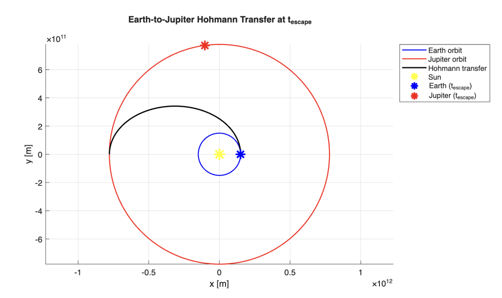
Figure 1: Heliocentric Hohmann transfer from Earth to Jupiter.
5 Conclusion
5.1 Discussion of Results
The results from this study show a feasible Earth-to-Jupiter transfer that is fuel-efficient but slow in time. The spacecraft’s heliocentric speed falls from 38,578 m/s at departure to only 7,413 m/s at Jupiter’s orbital radius, reflecting the substantial deceleration associated with outward Hohmann transfers. This explains why the mission’s Δv budget is dominated by the capture maneuver rather than departure: the departure burn required only 6,834 m/s, while capture required 10,870 m/s, nearly 60% more. Since Jupiter’s orbital speed (13,055 m/s) exceeds the spacecraft’s apoapsis speed (7,413 m/s), the spacecraft arrives with a hyperbolic excess velocity of 5,643 m/s. The transfer itself takes 997.9 days (2.73 yr), a direct consequence of Kepler’s third law applied to the large semi-major axis of the transfer ellipse; this long duration is the primary trade-off of the fuel-efficient Hohmann geometry compared with faster, higher-energy trajectories.
The computed SOI radius of 4.82×10¹⁰ m or 0.322 AU is large compared with the planet itself, about 670 Jupiter radii. This relatively large SOI, combined with the shallow 10.725° turn angle at departure versus the much steeper 144.40° turn at arrival, illustrates that Jupiter’s gravity dominates the terminal phase of the mission far more strongly than Earth’s does at departure, which is a natural consequence of Jupiter’s much larger μ and its greater distance from the Sun.
To assess the model’s accuracy, the results can be compared with the Galileo mission (D’Amario et al., 1992). Galileo was launched on 18 October 1989 and reached Jupiter on 7 December 1995, a flight of about 6.1 years compared with the 2.73 years of the direct Hohmann transfer computed here. This longer flight was due to its Venus–Earth–Earth gravity-assist (VEEGA) trajectory, which was needed because its upper stage could not provide the large departure energy of a direct transfer; the model’s departure requires v∞ = 8,794 m/s at Earth. At arrival, Galileo’s Jupiter orbit insertion burn was about 630 m/s (D’Amario et al., 1992), compared with 10,870 m/s in this model. Galileo was captured into a highly elliptical orbit with a period of about 200 days and a periapsis of about 4 Jupiter radii, whereas this model assumes a circular orbit at 2×10⁸ m. Capturing into a circular orbit requires removing almost all of the spacecraft’s excess energy, while an elliptical orbit only requires slowing it enough to stay bound to Jupiter. Galileo’s Io flyby just before insertion also reduced the burn it needed. This comparison suggests that the circular capture orbit, rather than the patched-conic approximation itself, is the main reason the model’s total Δv is so high.
Overall, the model shows the expected behaviour of an interplanetary transfer: a fuel-efficient but long-duration Hohmann transfer, with most of the Δv required for capture, and a relatively wide but manageable patched-conic boundary near the target planet.
5.2 Limitations
The patched-conic method treats each phase as an independent two-body problem, ignoring simultaneous gravitational effects from all three bodies. Moreover, Earth and Jupiter are assumed to be on circular, coplanar orbits, though both have small real eccentricities and inclinations. Additionally, departure and capture burns are modeled as instantaneous impulses rather than finite-thrust maneuvers, and perturbations such as solar radiation pressure, other planets, and Jupiter’s oblateness are neglected.
5.3 Future Extensions
In future work, a full n-body numerical propagation would capture simultaneous gravitational effects from the Sun, Earth, and Jupiter, giving a more accurate trajectory than the patched-conic approximation. Incorporating the true eccentricities and orbital inclinations of Earth and Jupiter, rather than assuming circular, coplanar orbits, would refine the launch-window and phasing calculations. Moreover, replacing impulsive burns with finite-thrust maneuver models would better represent real propulsion systems. Furthermore, the analysis could be extended to compare alternative trajectories, such as bi-elliptic transfers, to evaluate trade-offs between transfer time and fuel cost. Finally, adding perturbing forces, such as solar radiation pressure, would push the model closer to a mission-realistic trajectory design.
References
Danciu, B. (2023). Interplanetary mission design [Computer software]. MATLAB Central File Exchange. https://www.mathworks.com/matlabcentral/fileexchange/66192-interplanetary-mission-design
Danciu, B. (2026). Interplanetary trajectory [Computer software]. GitHub. https://github.com/bogdandanciu/interplanetary_trajectory
Lutze, F. H. (n.d.). Summary of patched conic approximations [PDF]. Virginia Tech, Aerospace and Ocean Engineering. Retrieved September 29, 2026, from https://archive.aoe.vt.edu/lutze/AOE4134/patchedconiceqs.pdf
Schaub, H. (n.d.). ScenarioPatchedConics. Basilisk. Retrieved September 29, 2026, from https://hanspeterschaub.info/basilisk/examples/scenarioPatchedConics.html
NASA. (2023). Chapter 4: Trajectories. NASA Science. https://science.nasa.gov/learn/basics-of-space-flight/chapter4-1/
Solar System Dynamics. (n.d.). Planetary physical parameters. NASA Jet Propulsion Laboratory. Retrieved September 29, 2026, from https://ssd.jpl.nasa.gov/planets/phys_par.html
Curtis, H. D. (2021). Orbital mechanics for engineering students (4th ed.). Butterworth-Heinemann. https://doi.org/10.1016/C2020-0-01873-6
Fidkowski, K., Atkins, E., & Powell, K. (2019). Course notes for Introduction to Aerospace Engineering. University of Michigan.
D’Amario, L. A., Bright, L. E., & Wolf, A. A. (1992). Galileo trajectory design. Space Science Reviews, 60, 23–78. https://doi.org/10.1007/BF00216849
Byrnes, D. V., & D’Amario, L. A. (1983). Interplanetary trajectory design for the Galileo mission. AIAA Paper 83-0099. https://ntrs.nasa.gov/citations/19830036690
Comparison of a simple patched conic trajectory code to commercially available software. AAS 07-160 (2007). NASA Technical Reports Server. https://ntrs.nasa.gov/api/citations/20070010447/downloads/20070010447.pdf
Reppert, T. (2006). Extending the patched-conic approximation to the restricted four-body problem [Undergraduate thesis]. Supervised by H. Schaub. https://hanspeterschaub.info/Papers/UnderGradStudents/Reppert2006.pdf
ScienceDirect. (n.d.). Patched conic [Topic overview]. Retrieved September 29, 2026, from https://www.sciencedirect.com/topics/engineering/patched-conic
About the author
Nour Saffar
Nour is a high school student with a strong interest in mathematics, chemistry, and engineering, particularly chemical engineering. Through her research project, Nour realized that although aerospace engineering had previously been her dream, she is now more interested in pursuing chemical engineering.
Academically, Nour has maintained a strong performance and has been part of her school’s Honor Roll. Outside the classroom, Nour is involved in athletics, STEM initiatives, and community activities. She is currently the captain of his school’s FIRST Robotics team, where she aims to create opportunities for students to explore engineering, robotics, and scientific problem-solving. Nour also enjoys writing, reading, and learning about different cultures and perspectives.