Relation Between Geometric Brownian Motion and ARIMA in the Prediction of Stock Prices

Introduction

In light of the instability of the economy today, stock prices are a concern. Whether one should liquidate one’s investments or not is the question on many minds. Many economists have used models in order to predict any trends that a stock might have in the future. Two examples of these models are ARIMA and Geometric Brownian Motion. Although they have the same goal as a model, the two have major differences in accuracy, operation, errors, functions, and variables.

The prediction models GBM and ARIMA share numerous similarities and differences. First of all, both of them are stochastic processes (Floyd and Hadjifrangiskou). In the scientific Brownian Motion, stochastic motion is the random motion of particles that is caused by random collisions with molecules (Floyd and Hadjifrangiskou). This is similar in economics. With both GBM and ARIMA(mostly GBM), the models use random fluctuations in data in order to predict the future of the stock. In finance, using Brownian Motion one can predict random movement of data over some time. Due to this random motion, one can determine a solid trend of data that can solidify the data in the future.

Both these models use intervals of time and the data points taken from each interval in order to forecast the price. Although usually, to get the most accuracy, one should use all points of data in order to make a “best fit line” prediction, the GBM model does not use all of the intervals. In stocks, if one takes a mean of data over certain periods of time, it is going to fluctuate throughout different time frames(Kong). Brownian Motion says that the stochasticity would remain 0 if it exceeds Brownian Motion, which is not related to what happens in stocks (Ermogenous). On the other hand, one disadvantage of GBM, similar to ARIMA, is that the randomness it calculates is shown as constant when, in reality, stock prices are always fluctuating and unpredictable due to news or events that change the projection(Kong).

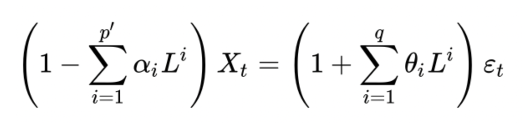
Methodology of ARIMA

ARIMA stands for Autoregressive Integrated Moving average. AR (Autoregression) is the changing of the variable that develops over its own prior values (Bajaj). I (Integrated) is the raw observations that make the time series able to become stationary (Bajaj). Data values are replaced by the difference between data values and previous values (Hayes and Stapleton). MA (Moving average) is the inclusion of dependency between an observation and an error from the moving average model of the ARIMA that is used with the lagged observations (Hayes and Stapleton). Moving average window is the period of time with the average data in that time period (Hayes and Stapleton). The top averages are then used to interpret and predict the next averages for the model.

• p is the parameter which represents the number of lag observations or what the time is that is passing(Hayes and Stapleton).
• d is the number of times that the raw observations are differenced that occur in the Integrated part of the model(Hayes and Stapleton).
• q is the size of the moving average window(Hayes and Stapleton).
• L is the component of the equation that uses another element of the time series in order to put out the previous element. This is also known as the lag operator.
•  θ_i is the representation of the parameter for the moving average (MA) of the equation.
• ε_t is the variable to show the error terms, which are independent variables, that are sampled from the normal distribution of the time series and spread out with an average equal to zero(Notation for ARIMA Models).
• ⍺_i are the parameters of the autoregressive component of the model (A) (Notation for ARIMA Models).
• X_t is a real number where t is an integer Figure 1 (Autoregressive integrated moving average)

Background of GBM

GBM derived from the Brownian Motion (Wiener Process), which was named by the botanist Robert Brown in 1828 when he was studying how pollen particles that are dispersed in water move randomly microscopically(Holton). The key component of Geometric Brownian Motion relates to that of Brownian Motion, randomness/erratic data. This realization of the stochastic process and its relation to pricing was uncovered by a French mathematician by the name of Louis Bachelier(Ermogenous). Bachelier published this idea in his doctoral thesis which was then looked at by Albert Einstein who then implemented this in thermodynamics(Holton). Later on in 1923, Norbert Wiener finalized the existence of the Brownian motion and its application in mathematics using mathematical theories to correlate the two(Holton). This is why Brownian motion is also sometimes called the “Wiener process”(Holton).

Methodology of GBM

An important part of the GBM model is that it will not spit out after doing its operations a negative value as the output(Kong). For example, when calculating the stock predictions, it cannot predict values and output it as a result in the form of a negative number(Kong). The solution of a problem solved by GBM is determined from the time prediction, which is represented by the t parameter. Predictions would be accurate in stock prices when one has a smaller time horizon/factor/period. Two hours in the future prediction would be more accurate than a prediction for five hours or two days in the future because there is data that is being observed over a shorter period so a comparison of data can be more evident. The W is the Brownian Motion (Wiener Process) itself. It is to represent the random motion, which is a key role in prediction using this model. Nu is shown for percent drift(Ross, 612-14). This is the average of how much the data is drifting and has changed from a baseline data point, which can be like an initial point of what to refer to for the change in data(Ross, 612-14).

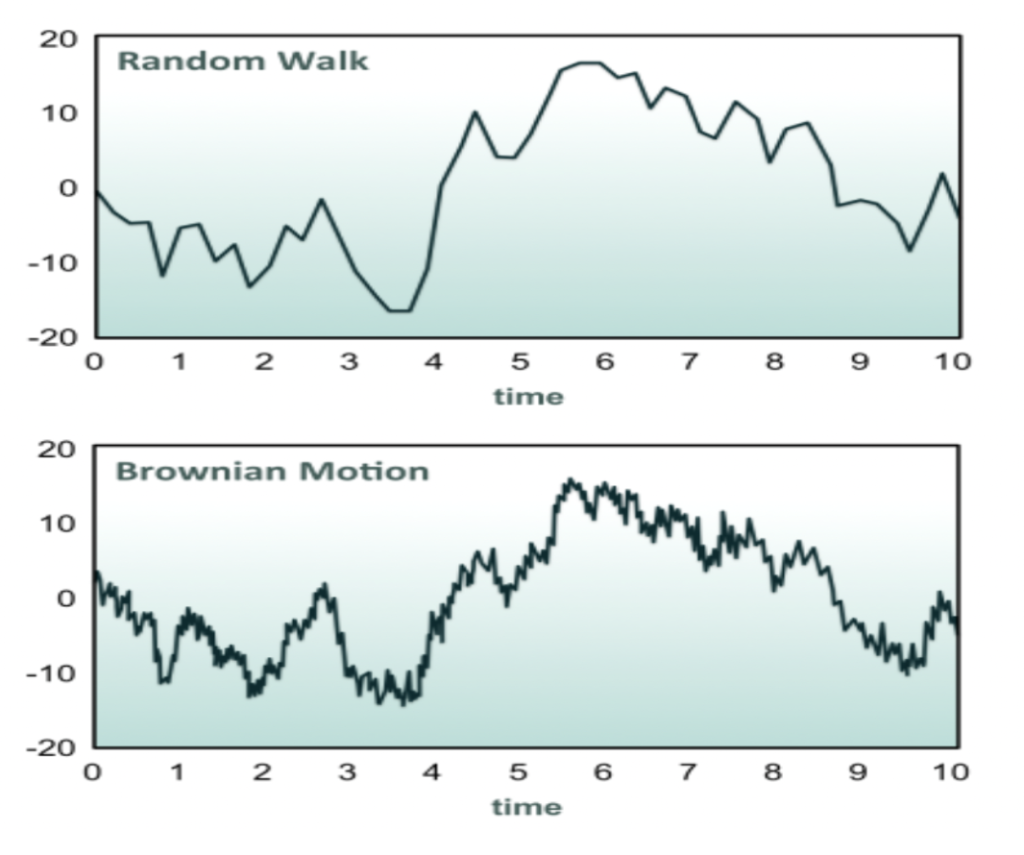
Note. Random Walk is a model that falls in the ARIMA model category, and Brownian motion model( Random walk model). The Brownian Motion Graph shows the fluctuation of data.

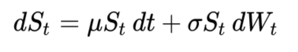
Note.

• S_t is the Stochastic Process that follows the Geometric Brownian Motion Model (Ermogenous).
• nu is the percent drift/error of the process(Herzog).
• σ is the volatility. In this case, GBM in finance, this is the rate at which the price of the stock will increase or decrease(Herzog).

Accuracy of GBM

As compared to ARIMA, GBM is more widely used for stock prediction due to its great accuracy. For stock price prediction, the geometric Brownian Motion Model uses an algorithm that begins by calculating the return value and then estimating the value of the data fluctuating and randomly changing (Farida Agustini et al.). Then the model uses all of that to predict the stock price forecast to help predict the prices for the user. The accuracy of the GBM is very strong and is around 95% (Farida Agustini et al.). This accuracy rate, also known as confidence level, is supported by the MAPE value (Farida Agustini et al.), where MAPE stands for mean absolute percentage error. Along with a high accuracy rate, the GBM process also outputs a MAPE value of ≤20%, which also supports the reliability of this process compared to others (journal of physics conference series) (Farida Agustini et al.). Another benefit of GBM is that the calculations of the model are simple, and it outputs the IV of the significance of the price of the stock (Kong).

Note.

• n is the sample size in the model
• “actual” is the actual data value of the model
• “forecast” is the forecasted data value of the model
• “| |” is representing the absolute value. This is used in the numerator and denominator of the equation.

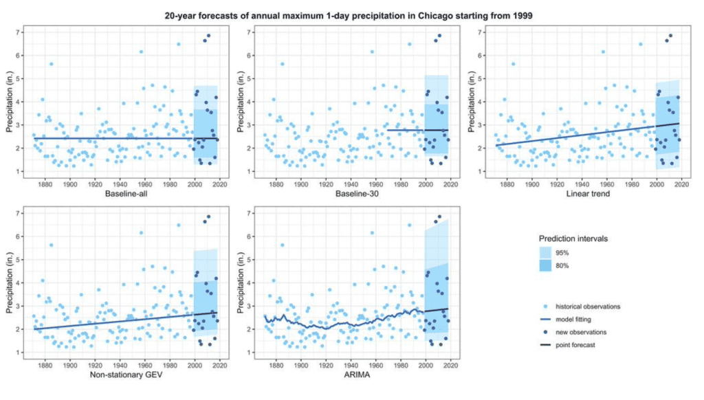
Note. On the bottom row of the graphs, the ARIMA model of the precipitation prediction is shown. The key also indicates that the darker points are the predictions. As seen in the graph, many of the points plotted are scattered due to the ARIMA showing the percent drift and fluctuation in forecasting data. The points that are located on the higher end of the y axis show that the prediction is stating a major change in precipitation due to some factors around the 2010 time frame.

Conclusion

GBM and ARIMA both have many things in common like their application in finance, stochastic motion, distribution, and their use of previous data points to make data predictions. On the other hand, the function, variables, and other uses differentiate both models evidently. Although the stochastic processes of GBM and ARIMA are used for predictions, GBM is greater in accuracy and reliability (Farida Agustini et al.).

References

“Autoregressive Integrated Moving Average.” Wikipedia, Wikimedia Foundation, 15 Oct. 2022, https://en.wikipedia.org/wiki/Autoregressive_integrated_moving_average.

Bajaj, Aayush. “Arima & Sarima: Real-World Time Series Forecasting.” Neptune.ai, 14 Nov. 2022, https://neptune.ai/blog/arima-sarima-real-world-time-series-forecasting-guide.

Business, Fuqua School of. “ Random Walk Model.” Random Walk Model, https://people.duke.edu/~rnau/Decision411_2007/411rand.htm.

Ermogenous, Angeliki. “Brownian Motion and Its Applications In The Stock Market.” University of Dayton ECommons, 2006, https://ecommons.udayton.edu/cgi/viewcontent.cgi?article=1010&context=mth_epu md.

Farida Agustini, W, et al. “Stock Price Prediction Using Geometric Brownian Motion.” Journal of Physics: Conference Series, vol. 974, 2018, p. 012047., https://doi.org/10.1088/1742-6596/974/1/012047.

Floyd, K A, and M Hadjifrangiskou. “Adhesion of Bacteria to Surfaces and Biofilm Formation on Medical Devices.” ScienceDirect, 2017, https://www.sciencedirect.com/topics/chemistry/brownian-motion. Accessed 30 Nov. 2022.

Hayes, Adam. “Autoregressive Integrated Moving Average (ARIMA).” Edited by Chip Stapleton, Investopedia, Investopedia, 24 June 2022, https://www.investopedia.com/terms/a/autoregressive-integrated-moving-average-ari ma.asp.

Herzog, Florian. “Stochastic Differential Equations – ETH Z.” Stochastic Differential Equations, 2013, https://ethz.ch/content/dam/ethz/special-interest/mavt/dynamic-systems-n-control/idsc-dam/Lectures/Stochastic-Systems/SDE.pdf.

Holton, Glyn. “Brownian Motion (Wiener Process).” GlynHolton.com, 10 Oct. 2016, https://www.glynholton.com/notes/brownian_motion/.

Kong, Yuxuan. “Geometric Brownian Motion – Mi.uni-Koeln.de.” Geometric Brownian Motion, May 2017, http://www.mi.uni-koeln.de/wp-znikolic/wp-content/uploads/2017/05/4_Geometric_Br ownian_Motion_28042017.pdf.

Lai, Yuchuan, and David A. Dzombak. “Use of the Autoregressive Integrated Moving Average (ARIMA) Model to Forecast Near-Term Regional Temperature and Precipitation.” AMS, vol. 35, no. 3, 1 Apr. 2020, pp. 959–976. “Notation for ARIMA Models.” SAS/ETS, July 2011.

Ross, Sheldon M. Introduction to Probability Models (Eleventh Edition). 11th ed., Academic Press, 2014.

Zach. “What Is Considered a Good Value for Mape?” Statology, 10 May 2021, https://www.statology.org/what-is-a-good-mape/.

---