

Author: Ruthvik Reddy Bommireddy
Mentor: Dr. Peter Kempthorne
Delhi Public School Bangalore North
Abstract
Economic time series are considered to be the economic barometers of the health of an economy. They provide information about the performance and stability of key economic indicators, such as inflation. Therefore, it is wise to try and forecast these variables.
In this paper, we implement time series modeling techniques using R programming language to analyze economic time series related to inflation and interest rates. Specifically, we apply simple and ARIMA models to forecast the Consumer Price Index (CPI).
To focus our analysis, we will apply our method of analysis to one CPI series, and then use the same method for the remaining CPI series. This will allow us to compare the accuracy of our models across different CPI series and identify any patterns or trends in the data.
The goal of this analysis is to compare the accuracy of simple and ARIMA models for forecasting CPI. We will use evaluation measures such as Mean Absolute Error (MAE) and Root Mean Squared Error (RMSE) to compare the performance of the two models. Our analysis will provide insights into which modeling technique is better suited for forecasting these economic variables.
1. Historical Time Series of Inflation in the US
1.1 Overview of Series
Our research analyses time series on consumer prices in the U.S. maintained by the St. Louis Federal Reserve. Specifically, we analyse three series:
- Consumer Price Index for All Urban Consumers: All Items in U.S. City Average (CPIAUCSL)
- Consumer Price Index for All Urban Consumers: All Items Less Food and Energy in U.S. City Average (CPILFESL)
- Consumer Price Index for All Urban Consumers: All Items Less Food and Energy in U.S. City Average (CPILFENS)
CPILFENS and CPIFESL are both CPI series produced by the BLS, but they differ in terms of their geographic coverage, scope of coverage, and methodology. Also, CPILFESL is seasonally adjusted and CPILFENS is not. These are all monthly time series from January 2011 to November 2022. The next section provides descriptions of the four series.
1.2 Series Descriptions
Reference : https://fred.stlouisfed.org/
1.2.1 Description of CPIAUCSL
Source: U.S. Bureau of Labor Statistics
Units:Index 1982-1984=100, Seasonally Adjusted Frequency: Monthly
CPIAUCSL stands for Consumer Price Index for All Urban Consumers: All Items. It is a measure of the average change over time in the prices paid by urban consumers for a basket of goods and services, including food, housing, clothing, transportation, and medical care, among others. The CPIAUCSL is produced by the United States Bureau of Labor Statistics and is used as an indicator of inflation in the US economy.
1.32 Description of CPILFESL
Source: U.S. Bureau of Labor Statistics Release: Consumer Price Index
Units: Index 1982-1984=100, Seasonally Adjusted Frequency: Monthly
CPILFESL stands for Consumer Price Index for All Urban Consumers: All Items Less Food and Energy. It is a measure of the average change over time in the prices paid by urban consumers for a basket of goods and services, excluding food and energy prices. This measure is used to gauge the underlying inflation trend in the US economy, as food and energy prices can be highly volatile and subject to seasonal changes that can obscure the overall inflation trend. CPIFESL focuses on a narrow range of goods and services, including food, housing, apparel, and transportation.
1.35 Description of CPILFENS
Source: U.S. Bureau of Labor Statistics Release: Consumer Price Index
Units: Index 1982-1984=100, Not Seasonally Adjusted Frequency: Monthly
The “Consumer Price Index for All Urban Consumers: All Items Less Food & Energy” is an aggregate of prices paid by urban consumers for a typical basket of goods, excluding food and energy. This measurement, known as “Core CPI,” is widely used by economists because food and energy have very volatile prices.CPILFENS covers a broad range of goods and services, including food, housing, clothing, transportation, and medical care.
1.4 Extract symbol list
To conduct our analysis, we used an R time series object named “economic_data2.” This quarterly time series spans from 2011-01-01 to 2022-11-30 and contains multiple columns representing the three Consumer Price Index (CPI) series: CPILFENS (Consumer Price Index for All Urban Consumers: All Items Less Food & Energy), CPIAUCSL (Consumer Price Index for All Urban Consumers: All Item), and CPILFESL (Consumer Price Index for All Urban Consumers: All Items Less Food and Energy). The R objects were created by importing data directly from the Federal Reserve Economic Data (https: //fred.stlouisfed.org/).
We can extract the individual time series from economic-data2 using the following code
list_symbols<- unique(economic_data2$symbol)2. Methodology
In this research paper, we investigated the time series properties of 3 CPI series : CPILFENS, CPIAUCSL, and CPILFESL.
Our approach was guided by the principles outlined in the book “Forecasting: Principles and Practice” by Rob J. Hyndman and George Athanasopoulos (Hyndman and Athanasopoulos, 2018). To perform the data analysis and modeling, we employed the functionality provided by the “fpp2” package in R. By applying the methodologies outlined in Hyndman’s book and implementing the “fpp2” package, we were able to conduct rigorous and robust time series analysis on the economic data.
To conduct our study, we first performed a series of exploratory data analysis by visually observing the time series plots and their seasonal plots, and the autocorrelation function (ACF). Subsequently, we used simple models , namely naive and drift, to forecast the data. Upon further investigation, we found that we can reject the null hypothesis that the time series are stationary for all three series, meaning their statistical properties change over time.
To transform the data into stationary time series, we applied first and second differencing. Next, we applied the auto.arima function from the forecast package in R to find the best fit model for each variable. For CPIAUCSL, the best model is ARIMA(0,1,1) with drift, indicating that the variable is influenced by its own one lagged value and has a linear trend over time. For CPILFENS, the best model is found to be ARIMA(2,1,0) with drift, indicating that the variable is influenced by its own two lagged values and has a linear trend over time. For CPILFESL, the best model is ARIMA(1,2,1), indicating that the variable is influenced by its own one lagged value , has a quadratic trend over time and is affected by a lagged moving average of order one.
We then applied root mean squared error (RMSE) , mean absolute error (MAE) , and mean absolute percentage error (MAPE). The results showed us that the ARIMA models provide forecasts for all three variables with relatively low error measures.
In the following section, we will delve into the detailed analyses of the three economic time series, namely CPIAUCSL, CPILFENS, and CPILFESL. This section will provide a comprehensive overview of the methodologies and the R code employed to generate the results. By including the R code, we aim to facilitate our readers to replicate the analyses presented in this paper or apply them to other time series data. We provide a practical resource for anyone who wishes to explore our methodologies further or extend the analyses to different time series datasets.
Through this detailed examination of the analyses and the inclusion of the R code, we hope that the insights gained from our research can be readily applied and built upon by the wider community.
3. Analysis of Consumer Price Index for All Urban Con- sumers: All Items Less Food and Energy in U.S. City Aver- age (CPILFESL)
3.1 Extract time series and plot the time plot, seasonal plot and auto- correlation function
First, extract series and create a ts object:
symbol1<- list_symbols[2]
data.symbol1<- filter(economic_data2, symbol==symbol1)
symbol1.ts<- ts(data.symbol1$price, frequency=12, start=c(2011,1))
Time Plot
autoplot(log((symbol1.ts)))+
  ggtitle("Time Plot")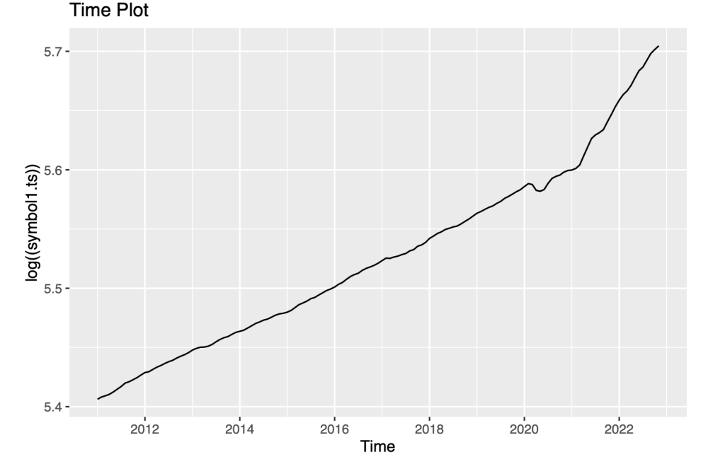
Upon examining the data, we have made several observations about the trends in CPILFESL:
Firstly, we noted that CPILFESL fell in the year 2020. This indicates a decrease in inflation, as a falling CPI suggests that prices for goods and services are decreasing.
Secondly, we observed a considerable increase in CPILFESL during the years 2021 and 2022. This indicates an increase in inflation, as the CPI is rising.
Thirdly, we noticed that before the year 2020, the index increased at a constant linear rate. This suggests a relatively stable inflation rate during this time period, with prices for goods and services increasing at a steady rate.
Finally, we observed that after 2020, the index rose at a much faster rate. This indicates a sudden increase in inflation during this time period, which could be due to a variety of factors such as changes in supply and demand, shifts in government policies, or other external factors.
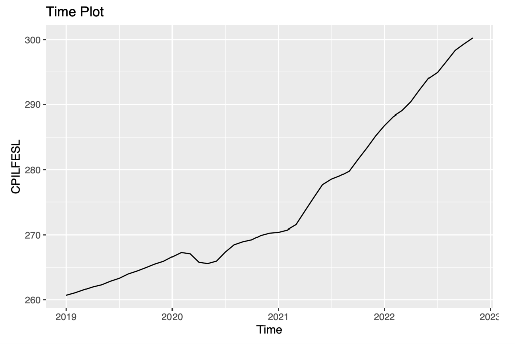
The main objective of predicting the index is to evaluate the sensitivity of our forecasting models to the use of data prior to the year 2020. Basically, we want to understand how the accuracy and reliability of our predictions are affected by the inclusion of data from and before 2020.
autoplot(window(symbol1.ts,start=c(2019,1)))+
  ggtitle("Time Plot") +
  ylab("CPILFESL")+
  xlab("Time")
Seasonal Time Plot :
A seasonal plot is a graphical representation of a time series that provides insights into its seasonal patterns. It helps identify repeating patterns or cycles within the data that occur over fixed time intervals, such as daily, monthly, or yearly patterns.
We use the following R code to plot the seasonal plot
ggseasonplot(symbol1.ts, polar= TRUE)+
  ylab("CPILFESL")+
ggtitle("Seasonal Plot: CPILFESL")
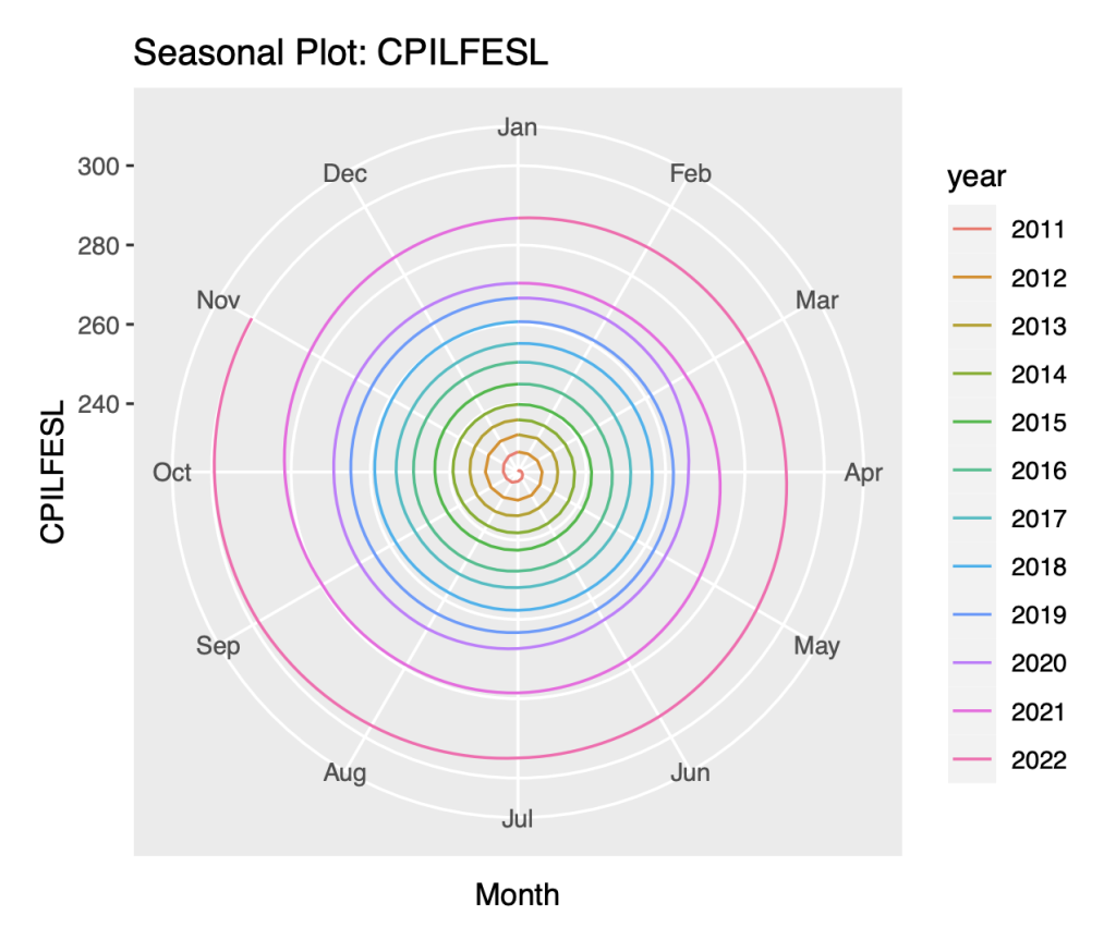
The seasonal plot is implemented by the “fpp2” package. It is a one-of-a-kind data visualisation technique that represents time series values in polar coordinates. By using polar coordinates, the seasonal plot provides a compact and simple representation of the seasonal patterns in the data. In this plot, the angle corresponds to the month-of-year, while the radius represents the time from the beginning of the series.
we have made the following observations:
Firstly, we noted that there is a large jump in the CPILFESL variable every year. This indicates that there is a significant change in the rate of inflation from one year to the next. This could be due to a variety of factors.
Secondly, we observed that there is no overlap in the data of the seasons. This means that the data points for each season are distinct and do not overlap with each other. This pattern could have important implications for our analysis, as it suggests that there may be seasonal trends or patterns that are unique to each season.
Autocorrelation and white noise :
ggAcf(symbol1.ts)+
  ggtitle(symbol0)
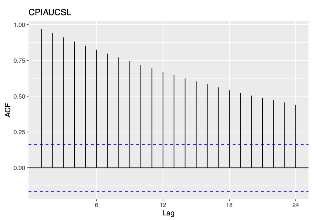
Based on our observations of the data, we have identified several important patterns that provide insight into the nature of the time series:
Firstly, we noted that there was a slow decrease in the autocorrelation function (ACF) as the lags increased.
Secondly, we compared the spikes in the ACF to the expected values for a white noise series. Specifically, we expected 95% of the spikes in the ACF to lie within the range of ±2/ T, where T is the length
of the time series. In this case, T is equal to 11*12, or 132. This means that we would expect the spikes in the ACF to lie within the range of ±0.17
However, we found that the spikes in the ACF actually lie above +0.17 and cross the blue bounds. This indicates that the series is not white noise, as there is significant correlation between the data points that cannot be explained by random chance alone.
The observed ACF pattern, where the autocorrelation gradually decreases as the lag increases, is typical of non-stationary time series. This pattern is often observed in time series models such as random walks. In section 3.2, we investigate the characteristics of non-stationary time series, particularly random walks, and analyze their behavior using the naive and drift models. Further, section 3.2 provides insights into the suitability of these models for capturing the dynamics of non-stationary time series, such as random walks, and sheds light on their capabilities to forecast in such situations.
3.2 Evaluate simple forecast models
3.2.1 Random walk with naive
Using the R package “fpp2”, let’s apply the naive method
symbol1.ts.naive=naive(symbol1.ts)
autoplot(symbol1.ts.naive)+
ylab(symbol1)+
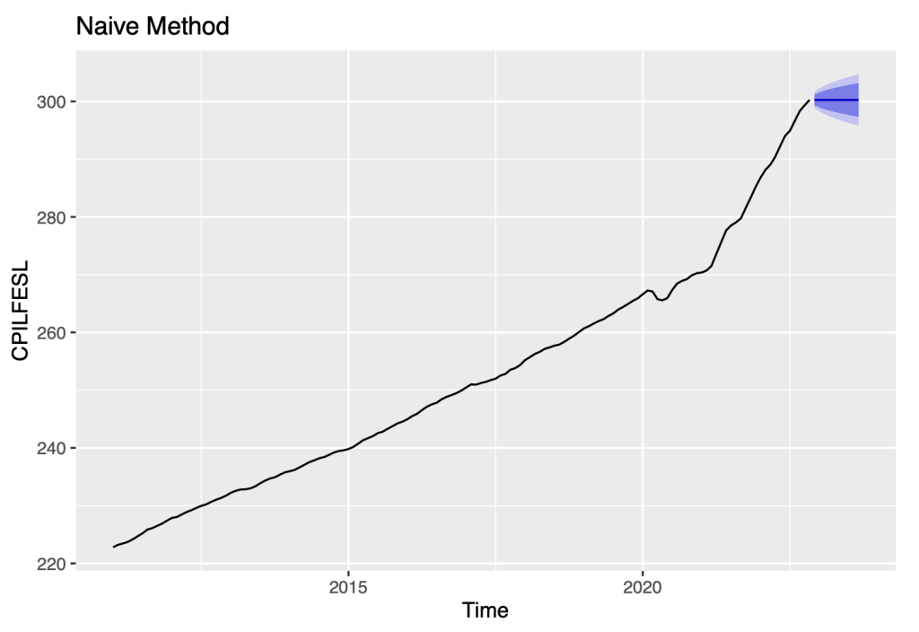
ggtitle("Naive Method")
checkresiduals(symbol1.ts.naive)
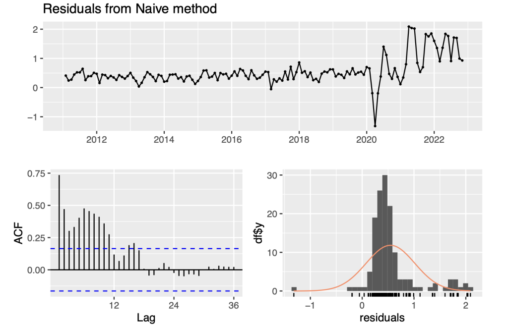
##
##  Ljung-Box test
##
## data:  Residuals from Naive method
## Q* = 340.41, df = 24, p-value < 2.2e-16
##
## Model df: 0.   Total lags used: 24
The naive method of forecasting assumes that all future forecast values will be the same as the previous or last observation. However, this method is not useful
Regarding the seasonal naive method, this approach is only useful when the data is seasonal in nature, which is not the case for this particular dataset. Instead, the data appears to exhibit more of a trend-like pattern over time. Therefore, utilizing the seasonal naive method would not provide any meaningful insights or forecasts.
To ensure the adequacy of the naive model in capturing the underlying patterns of the non-stationary time series, we conducted a residual analysis. Residuals are the differences between the observed values and the corresponding model predictions. Analyzing the residuals allows us to assess the model’s ability to capture the remaining variation in the data.
In this analysis, we utilized the checkresiduals() function which provides various plots and tests to evaluate the model’s residuals. These plots and tests help in determining whether the model adequately captures the inherent patterns and randomness in the time series data.
By examining the plots, such as the autocorrelation function (ACF) and the histogram of residuals, we can assess if the residuals exhibit any remaining patterns or systematic behavior. Ideally, the residuals should be uncorrelated, normally distributed, and have constant variance.
In addition to visual inspection, the checkresiduals() function also performs statistical tests, including the Ljung-Box test, to check for significant autocorrelation in the residuals. A significant autocorrelation indicates that the model fails to capture some underlying structure in the data.
Upon analyzing the data, we have observed that the variability of the residuals is relatively low in the first half of the series, but it increases in the second half. This pattern indicates that taking the logarithms of the series is appropriate for applying stationary time series models. This approach can help to stabilize the variance of the data and make it easier to apply various statistical techniques.
After examining the data, we have found that taking logarithms does not seem to improve the stationarity of the series. However, we found that taking the second differences of the series, as opposed to the first differences, does lead to greater stationarity. This suggests that the trend in the data is not linear and may require more complex modeling techniques.
Now, we will check the errors of the naive method
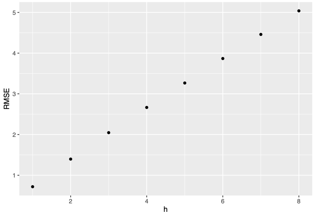
e <- tsCV(symbol1.ts, forecastfunction=naive, h=8)
# Compute the RMSE values and remove missing values
rmse <- sqrt(colMeans(eˆ2, na.rm = T))
# Plot the RMSE values against the forecast horizon data.frame(h = 1:8, RMSE = rmse) %>%
ggplot(aes(x = h, y = RMSE)) + geom_point()
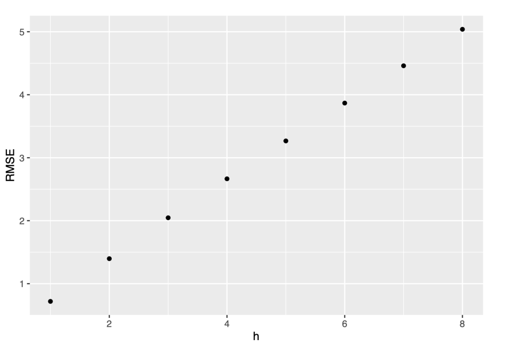
Throughout our analysis, we will provide RMSE values that are directly comparable to the original time series. This enables us to gauge the level of accuracy achieved by the forecasting models and make informed assessments about their suitability for practical applications and decision-making processes.
Upon examining the forecasting results, it becomes clear that the forecast error tends to increase as the forecast horizon increases. This means that the accuracy of our predictions tends to decrease as we try to forecast further into the future.
This is quite common because as we predict further into the future, forecasting becomes increasingly difficult due to uncertainty and variability of the outcomes.
e <- tsCV(symbol1.ts, forecastfunction = naive, h=1)
sqrt(mean(eˆ2, na.rm=TRUE))
## [1] 0.7189534
sqrt(mean(residuals(naive(symbol0.ts))ˆ2, na.rm=TRUE))
## [1] 0.9239518
The “tsCV” function is a useful tool for evaluating the accuracy of a time series forecasting model. It stands for “time series cross-validation” and is used to estimate the forecast error of a model. The “tsCV” function computes the forecast errors by dividing the time series data into training and testing sets. It fits the model to the training set and generates forecasts for the corresponding test set. The forecast errors are then calculated by comparing the predicted values to the actual values in the test set.
Comparing the cross-validation error to the RMSE of the residuals provides a way of assessing the model’s performance. The residuals are the differences between the observed values and the corresponding one-step predictions generated by the model. These residuals represent the in-sample prediction errors.
Ideally, the cross-validation error should be smaller than the RMSE of the residuals. This suggests that the model performs well not only on the data it was trained on but also on unseen data. If the cross- validation error is larger than the RMSE of the residuals, it indicates that the model may be overfitting the training data.
In this case, the RMSE of the cross-validation error is smaller than the RMSE of the residuals, suggesting the model performs quite well.
3.2.2 Random walk with drift
We now apply the drift method
autoplot(rwf(symbol1.ts, drift=TRUE),
    series="Drift")+
ylab(symbol1)+
  ggtitle("Drift Method")
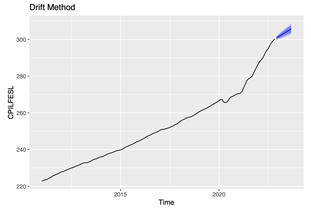
Here, we are referring to a forecasting method known as the drift method. The drift method involves taking the last observation of the data and adding to it the amount of change over time (i.e., the drift) of the data. The resulting value is then used as a forecast for future time periods.
The drift component of the data is a measure of how much the data tends to increase or decrease over time. By using this drift into the forecast, we are able to account for the overall trend in the data and make more accurate predictions about future values.
fit0 = rwf(symbol1.ts, drift=TRUE)
summary(fit0)

##
## Forecast method: Random walk with drift
##
## Model Information:
## Call: rwf(y = symbol1.ts, drift = TRUE)
##
## Drift: 0.5455  (se 0.0394)
## Residual sd: 0.47
##
## Error measures:
##                         ME      RMSE       MAE
## Training set -6.605036e-15 0.4683447 0.2966886 -0.007742377 0.1129022
##                    MASE      ACF1
## Training set 0.04767245 0.7353021
##
## Forecasts:
##
## Dec 2022
## Jan 2023
## Feb 2023
## Mar 2023
## Apr 2023
## May 2023
## Jun 2023
## Jul 2023
## Aug 2023
## Sep 2023
Point Forecast    Lo 80    Hi 80    Lo 95    Hi 95
      300.8065 300.2020 301.4109 299.8821 301.7309
      301.3520 300.4942 302.2098 300.0401 302.6639
      301.8974 300.8432 302.9517 300.2851 303.5097
      302.4429 301.2214 303.6644 300.5748 304.3111
      302.9884 301.6180 304.3588 300.8926 305.0842
      303.5339 302.0276 305.0401 301.2303 305.8375
      304.0794 302.4469 305.7118 301.5828 306.5759
      304.6248 302.8738 306.3758 301.9469 307.3027
      305.1703 303.3069 307.0337 302.3205 308.0201
      305.7158 303.7451 307.6865 302.7019 308.7297
checkresiduals(fit0)
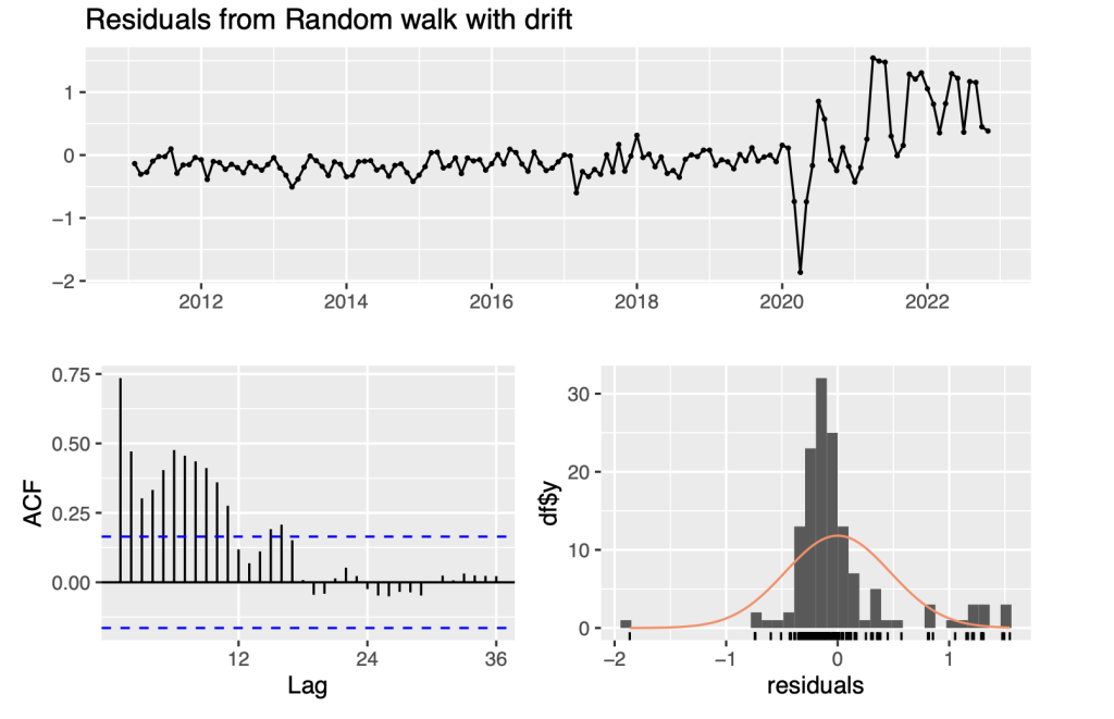
##
##  Ljung-Box test
##
## data:  Residuals from Random walk with drift
## Q* = 340.41, df = 23, p-value < 2.2e-16
##
## Model df: 1.   Total lags used: 24

accuracy(fit0)
##                         ME      RMSE       MAE          MPE      MAPE
## Training set -6.605036e-15 0.4683447 0.2966886 -0.007742377 0.1129022
##                    MASE      ACF1
## Training set 0.04767245 0.7353021
The output from the “fit0” model provides us with point forecasts and prediction intervals using the “rwf” function. The “rwf” function calculates point forecasts based on the random walk with drift model and provides prediction intervals that capture the uncertainty of the forecasts. We utilized the checkresiduals() function which provides various plots and statistical tests to evaluate the new model’s residuals. These plots and tests help us determine whether the model adequately fits the data.
We have made the following important observations :
Firstly, we can see that as the forecast horizon (h) increases, the width of the prediction intervals also increases. This widening of the prediction intervals is expected because forecasting becomes more challenging as we project further into the future. The increased uncertainty over longer time horizons results in wider intervals to account for the potential variability in the forecasted values.
Secondly, the estimated drift coefficient is 0.5455 with a standard error of 0.0394. This indicates that the time series has a linear trend over time. Also, the residual standard deviation is 0.47, which represents the average magnitude of the differences between the observed values and the forecasted values.
Thirdly, the RMSE (root mean squared error) is 0.4683447, indicating the average magnitude of the forecast errors. The MAE (mean absolute error) is 0.2966886, representing the average absolute magnitude of the errors. The MPE (mean percentage error) is -0.007742377. The MAPE (mean absolute percentage error) is 0.1129022, reflecting the average percentage deviation of the forecasts. The MASE (mean absolute scaled error) is 0.0476724. The ACF1 (first-order autocorrelation coefficient) is 0.7353021, suggesting a relatively high autocorrelation.
Finally, the test statistic (Q*) is 340.41, indicating significant evidence of autocorrelation.
Overall, the output suggests that while the random walk with drift model captures the linear trend in the time series, there are still autocorrelations that the model does not account for. Development of ARIMA models will address this issue below.
Now let’s check the errors in drift method
e <- tsCV(symbol1.ts, forecastfunction=naive, h=8)
# Compute the RMSE values and remove missing values
rmse <- sqrt(colMeans(eˆ2, na.rm = T))
# Plot the RMSE values against the forecast horizon
data.frame(h = 1:8, RMSE = rmse) %>%
ggplot(aes(x = h, y = RMSE)) + geom_point()
e <- tsCV(symbol1.ts, rwf, drift=TRUE, h=1)
sqrt(mean(eˆ2, na.rm=TRUE))
## [1] 0.4723834
sqrt(mean(residuals(rwf(symbol1.ts, drift=TRUE))ˆ2, na.rm=TRUE))
## [1] 0.4683447
Comparing the RMSE values of drift and naive, we can see that the RMSE for the drift model (0.4683447) is lower than the RMSE for the naive model (0.9239518). This indicates that the drift model performs better in terms of forecast accuracy, as it has a lower average magnitude of errors compared to the naive model.
The lower RMSE in the drift model suggests that incorporating the linear trend (drift) in the forecast model improves its forecasting capability. The drift model takes into account the systematic change in the time series over time, resulting in more accurate forecasts compared to the naive model, which assumes no drift.
Therefore, based on the RMSE values, the drift model is preferred over the naive model for forecasting this time series.
3.3 Fit ARIMA models
The null hypothesis for our analysis is that the time series data is stationary. This means that the statistical properties of the data, such as the mean and variance, remain constant over time. To analyze this time series data, we will use an auto-regressive integrated moving average (ARIMA) model that will be used to identify trends and patterns in the data, and make predictions about future values.
In the R programming language, we can use the auto.arima() function to identify and specify a fitted ARIMA model for our data. This function automates the process of selecting the appropriate model by searching for the best-fitting model based on a variety of statistical criteria.
library(urca)
goog %>% ur.kpss() %>% summary()
##
## #######################
## # KPSS Unit Root Test #
## #######################
##
## Test is of type: mu with 7 lags.
##
## Value of test-statistic is: 10.7223
##
## Critical value for a significance level of:
##                 10pct  5pct 2.5pct  1pct
## critical values 0.347 0.463  0.574 0.739
Based on our statistical analysis, we have found that we can reject the null hypothesis that the time series or data is stationary. This conclusion is based on the fact that the value of our test statistic was found to be higher than the critical values.
A stationary time series or data is one in which the statistical properties such as mean and variance do not change over time. In contrast, a non-stationary time series or data has statistical properties that change over time. The fact that we have rejected the null hypothesis indicates that the time series or data under consideration is not stationary, meaning that its statistical properties change over time.
We will now apply the technique of differencing. By doing so, we can improve the accuracy and reliability of our analysis, and make more informed decisions based on modeling a transformation of the time series that satisfies a test for consistency with being stationary.
The KPSS (Kwiatkowski-Phillips-Schmidt-Shin) test is a statistical test used to assess the stationarity of a time series. Stationarity refers to the property of a time series where its statistical properties (such as mean and variance) remain constant over time.
In the context of the KPSS test, the null hypothesis assumes that the time series is stationary. If the test statistic exceeds the critical value, it indicates evidence against the null hypothesis. This implies that the series is likely non-stationary.
Now let’s examine the output of the KPSS test
library(urca)
symbol1.ts %>% ur.kpss() %>% summary()
##
## #######################
## # KPSS Unit Root Test #
## #######################
##
## Test is of type: mu with 4 lags.
##
## Value of test-statistic is: 2.8269
##
## Critical value for a significance level of:
##                 10pct  5pct 2.5pct  1pct
## critical values 0.347 0.463  0.574 0.739

ndiffs(symbol1.ts)
## [1] 2
# for whole series, ndiffs() suggests second order differencing.
The test statistic value is 2.8269, and it is compared against critical values at different significance levels. The critical values at significance levels of 10%, 5%, 2.5%, and 1% are 0.347, 0.463, 0.574, and 0.739, respectively.
In this case, the test statistic value of 2.8269 exceeds all the critical values. Therefore, we reject the null hypothesis of stationarity, suggesting that the time series may not be stationary.
The ndiffs() function is also applied to determine the number of differences required to achieve station- arity for the whole series. In this case, ndiffs(symbol1.ts) suggests second-order differencing to achieve stationarity.
library(urca)
symbol1.ts[1:108] %>% ur.kpss() %>% summary()
##
## #######################
## # KPSS Unit Root Test #
## #######################
##
## Test is of type: mu with 4 lags.
##
## Value of test-statistic is: 2.2539
##
## Critical value for a significance level of:
##                 10pct  5pct 2.5pct  1pct
## critical values 0.347 0.463  0.574 0.739
ndiffs(symbol1.ts[1:108])
## [1] 2
# for whole series, ndiffs() suggests second order differencing.
Above, the subset symbol1.ts[1:108] is used, which means only the first 108 observations are consid- ered. Previously, the entire symbol1.ts time series was analyzed.
The time frame of 1:108 was specifically selected to fit the time series data, which includes inflation rates up until the year 2020. We identified a kink in the Consumer Price Index (CPI) at a certain point within this time frame, and we used this point as a cutoff for our analysis. By doing so, we were able to focus our analysis on a relevant and informative subset of the data, which allowed us to make more accurate and meaningful observations about inflation trends over time.
library(urca)
symbol1.ts[1:108] %>% ur.kpss() %>% summary()
The output shows that in both cases, the test statistic exceeds the critical values, indicating evidence against the null hypothesis of stationarity. The ndiffs() function suggests that 2 differences may be needed to achieve stationarity in both cases.
Overall, the difference in the output is primarily due to the subset of the time series under consider- ation, while the interpretation of the test results remains the same.
Let’s now apply the kpss test for the original series, for the first difference series and second difference series to compare them side by side
##
## #######################
## # KPSS Unit Root Test #
## #######################
##
## Test is of type: mu with 4 lags.
##
## Value of test-statistic is: 2.8269
##
## Critical value for a significance level of:
##                 10pct  5pct 2.5pct  1pct
## critical values 0.347 0.463  0.574 0.739
##
## #######################
## # KPSS Unit Root Test #
## #######################
##
## Test is of type: mu with 4 lags.
##
## Value of test-statistic is: 1.2285
##
## Critical value for a significance level of:
##                 10pct  5pct 2.5pct  1pct
## critical values 0.347 0.463  0.574 0.739

# KPSS test for the first-difference series
symbol1_diff1 <- diff(symbol1.ts)
kpss_diff1 <- ur.kpss(symbol1_diff1)
summary(kpss_diff1)
##
## #######################
## # KPSS Unit Root Test #
## #######################
##
## Test is of type: mu with 4 lags.
##
## Value of test-statistic is: 0.0269
##
## Critical value for a significance level of:
##                 10pct  5pct 2.5pct  1pct
## critical values 0.347 0.463  0.574 0.739
# KPSS test for the second-difference series
symbol1_diff2 <- diff(symbol1.ts, differences = 2)
kpss_diff2 <- ur.kpss(symbol1_diff2)
summary(kpss_diff2)

##
## #######################
## # KPSS Unit Root Test #
## #######################
##
## Test is of type: mu with 4 lags.
##
## Value of test-statistic is: 0.0269
##
## Critical value for a significance level of
##                 10pct  5pct 2.5pct  1pct
## critical values 0.347 0.463  0.574 0.739
In the first case, we can observe that the test statistic for the original series (2.8269) is greater than the critical values at all significance levels. This suggests that the original series is non-stationary.
However, when we take the first difference of the series, the test statistic decreases to 1.2285. Although it is still higher than the critical values, it indicates a lower degree of non-stationarity compared to the original series.
Finally, the second-difference series exhibits a significantly lower test statistic of 0.0269, which is much smaller than the critical values. This indicates that the second-difference series can be considered stationary.
Overall, the KPSS test results suggest that the second-difference series shows the closest approxima- tion to stationarity among the three tested series.
library(urca)
# KPSS test for the original time series
kpss_original <- ur.kpss(symbol1.ts[1:108])
summary(kpss_original)
##
## #######################
## # KPSS Unit Root Test #
## #######################
##
## Test is of type: mu with 4 lags.
##
## Value of test-statistic is: 2.2539
##
## Critical value for a significance level of:
##                 10pct  5pct 2.5pct  1pct
## critical values 0.347 0.463  0.574 0.739

# KPSS test for the first-difference time series
symbol1_diff1 <- diff(symbol1.ts[1:108])
kpss_diff1 <- ur.kpss(symbol1_diff1)
summary(kpss_diff1)

##
## #######################
## # KPSS Unit Root Test #
## #######################
##
## Test is of type: mu with 4 lags.
##
## Value of test-statistic is: 0.54
##
## Critical value for a significance level of:
##                 10pct  5pct 2.5pct  1pct
## critical values 0.347 0.463  0.574 0.739

# KPSS test for the second-difference time series
symbol1_diff2 <- diff(symbol1.ts[1:108], differences = 2)
kpss_diff2 <- ur.kpss(symbol1_diff2)
summary(kpss_diff2)

##
## #######################
## # KPSS Unit Root Test #
## #######################
##
## Test is of type: mu with 4 lags.
##
## Value of test-statistic is: 0.0241
##
## Critical value for a significance level of:
##                 10pct  5pct 2.5pct  1pct
## critical values 0.347 0.463  0.574 0.739
In the first case, the test statistic (2.2539) is larger than the critical values at all significance levels. This indicates that we can reject the null hypothesis, suggesting that the original series is non-stationary. In the second case, The test statistic (0.54) is smaller than the critical values at all significance levels. This suggests that we cannot reject the null hypothesis of stationarity for the first-difference series. Thus,
the first-difference series is considered stationary.
In the third case, The test statistic (0.0241) is significantly smaller than the critical values at all
significance levels. This suggests that we cannot reject the null hypothesis of stationarity for the second- difference series.
The first differenced series is consistent with stationarity when only the first 108 values are included in the series. The apparent evidence for second differences with the entire series is , perhaps, due to the high volatility of the series after period 108.
Now, let’s apply the auto.arima() function and the checkresiduals() function
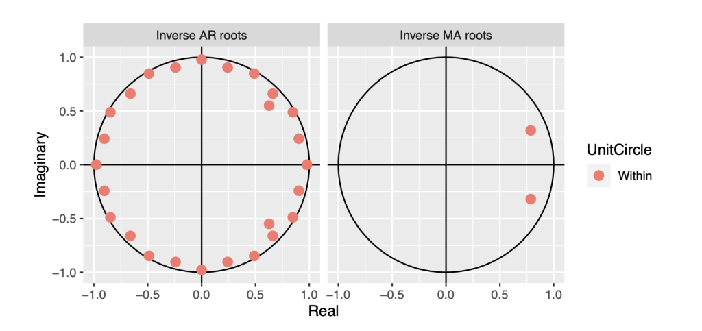
symbol1.ts.arima<- auto.arima(symbol1.ts)
summary(symbol1.ts.arima)
## Series: symbol1.ts
## ARIMA(2,2,2)(0,0,2)[12]
##
## Coefficients:
##          ar1      ar2      ma1     ma2     sma1     sma2
##       1.3288  -0.7466  -1.7074  0.8814  -0.2547  -0.1773
## s.e.  0.0785   0.0702   0.0625  0.0780   0.0988   0.0937
##
## sigma^2 = 0.07624:  log likelihood = -17.12
## AIC=48.24   AICc=49.08   BIC=68.88
##
## Training set error measures:
##                      ME      RMSE       MAE         MPE       MAPE       MASE
## Training set 0.01957902 0.2682821 0.1744252 0.006985389 0.06737252 0.02802695
##                   ACF1
## Training set 0.0259118
checkresiduals(symbol1.ts.arima)
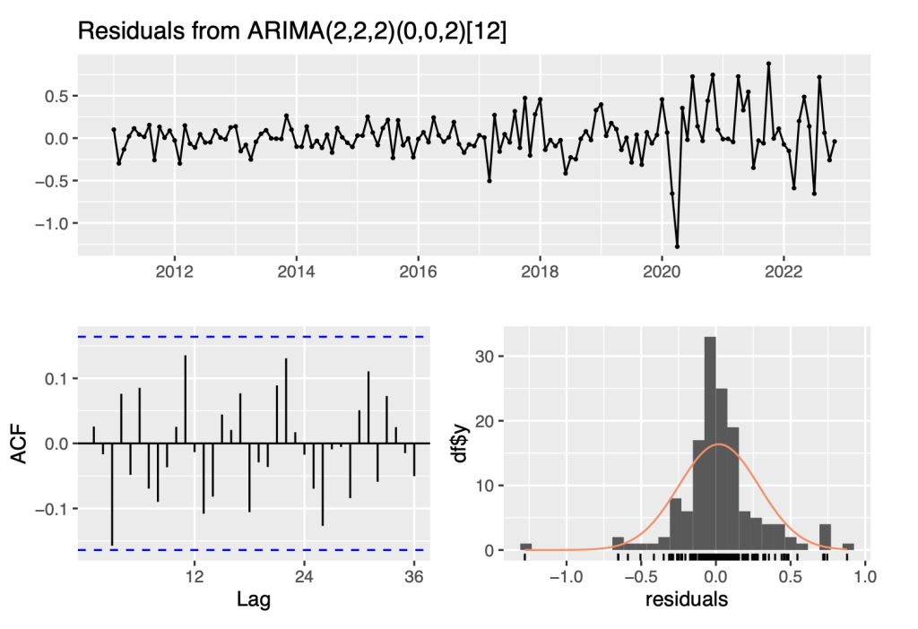
##
##  Ljung-Box test
##
## data:  Residuals from ARIMA(2,2,2)(0,0,2)[12]
## Q* = 22.222, df = 18, p-value = 0.2223
##
## Model df: 6.   Total lags used: 24
Seasonal ARIMA models are denoted by the notation ARIMA(p, d, q)(P, D, Q)[h], where the seasonal differences of order D are incorporated using the ARMA(P, Q) terms.
In this notation, the lowercase letters (p, d, q) represent the non-seasonal components of the model. The parameter ‘p’ denotes the order of the autoregressive (AR) component, which captures the de- pendence of the current observation on its previous values. The parameter ‘d’ represents the order of differencing required to achieve stationarity in the non-seasonal part of the series. The parameter ‘q’ indicates the order of the moving average (MA) component, which models the dependence of the current observation on the residual errors from previous observations.
On the other hand, the uppercase letters (P, D, Q) represent the seasonal components of the model. The parameter ‘P’ denotes the order of the seasonal autoregressive (SAR) component, which captures the dependence of the current observation on its previous seasonal values. The parameter ‘D’ represents the order of differencing required to achieve stationarity in the seasonal part of the series. The parameter ‘Q’ indicates the order of the seasonal moving average (SMA) component, which models the dependence of the current observation on the residual errors from previous seasonal observations.
The parameter ‘h’ represents the forecast horizon, indicating the number of future time steps for which we want to generate forecasts.
The output of the auto.arima() function suggests an ARIMA(2,2,2)(0,0,2)[12] model for the time series data. In this notation, the first set of numbers (2,2,2) represents the non-seasonal components of the ARIMA model. Specifically, it indicates that the model includes an autoregressive (AR) term of order 2, a differencing (I) term of order 2, and a moving average (MA) term of order 2. The second set of numbers (0,0,2) represents the seasonal components of the ARIMA model. In this case, the model includes a seasonal moving average (SMA) term of order 2. The seasonal terms account for the patterns and fluctuations that occur at regular intervals (in this case, with a period of 12).
Additionally, the p-value of the Ljung Box test is larger than 0.05. Therefore, we fail to reject the null hypothesis of no autocorrelation. This suggests that the residuals of the ARIMA model do not exhibit significant autocorrelation, supporting the adequacy of the model in capturing the remaining patterns in the data. Also, ACF does not cross the blue lines, suggesting that there is no significant autocorrelation in the residuals. It indicates that the model has adequately captured the underlying patterns in the data.
Now, let’s apply the auto.arima() function and the checkresiduals() function for the subset of the original series
symbol1.ts.arima<- auto.arima(symbol1.ts[1:108])
summary(symbol1.ts.arima)
## Series: symbol1.ts[1:108]
## ARIMA(1,2,1)
##
## Coefficients:
##          ar1      ma1
##       0.1956  -0.9525
## s.e.  0.1014   0.0344
##
## sigma^2 = 0.02133:  log likelihood = 55.94
## AIC=-105.88   AICc=-105.64   BIC=-97.89
##
## Training set error measures:
##                       ME      RMSE       MAE         MPE       MAPE    MASE
## Training set 0.008633132 0.1433159 0.1138458 0.003132918 0.04679805 0.28179
##                      ACF1
## Training set -0.009711438
checkresiduals(symbol1.ts.arima)
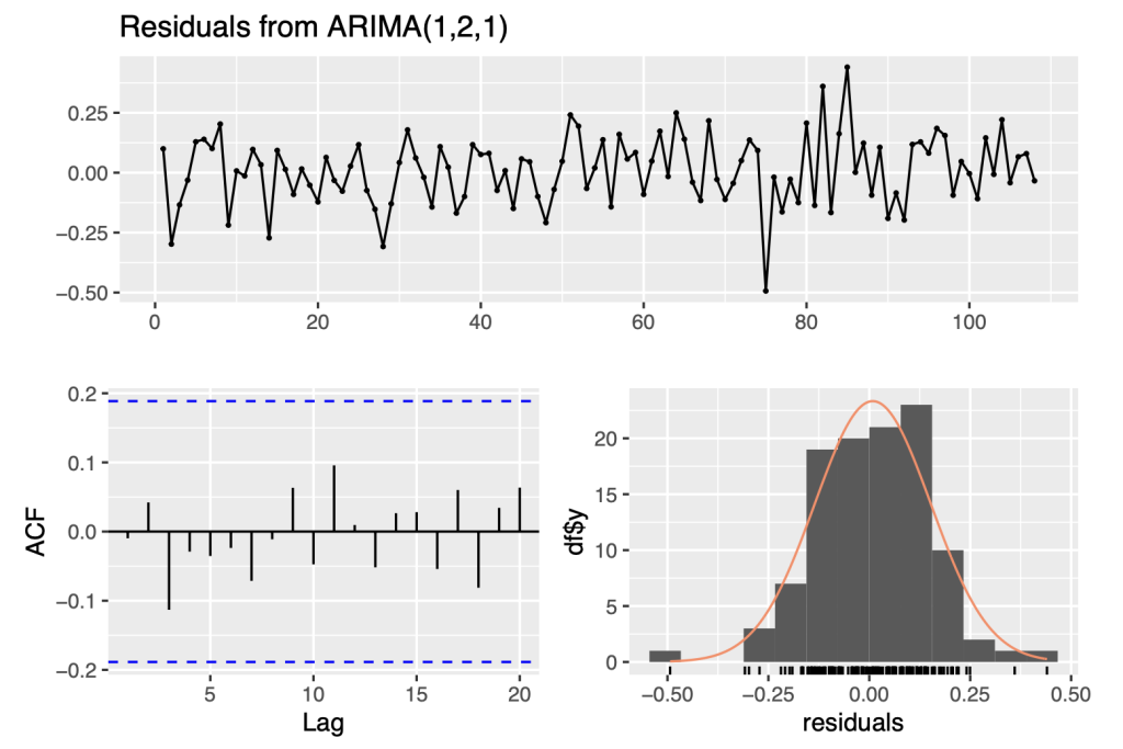
##
##  Ljung-Box test
##
## data:  Residuals from ARIMA(1,2,1)
## Q* = 3.3287, df = 8, p-value = 0.9121
##
## Model df: 2.   Total lags used: 10
The analysis above suggests that the data follows an ARIMA(1,2,1) model.The ARIMA notation consists of three numbers representing the number of autoregressive, integrated, and moving average terms, respectively. For this data, the model is ARIMA(1,2,1), meaning there is one autoregressive term, two integrated terms, and one moving average term. The seasonal components (P, D, Q) are not present, suggesting that the model does not capture any seasonal patterns.
This ARIMA(1,2,1) model is appropriate for the data based on the patterns that we observed in the data. These patterns suggest that there is a significant amount of correlation between the data points, and that this correlation decreases over time. By using this model, we can effectively capture these patterns and make accurate predictions about future trends in the data.
Comparison of the output of the symbol1.ts model with the symbol1.ts [1:108] model :
In terms of the RMSE, the second model (symbol1.ts [1:108]) has a lower value (0.1433159) compared to the first model (symbol1.ts) with a higher RMSE (0.2682821). This suggests that the second model provides a better fit to the data in the subset symbol1.ts [1:108] than the first model does to the entire symbol1.ts series.
Additionally, we can consider the Ljung-Box test results. The second model has a lower Ljung-Box test statistic (3.3287) compared to the first model (22.222), suggesting a better fit in terms of residual autocorrelation. In both the models, the p value is quite high, indicating that there is no evidence of significant autocorreltion.
Taking into account the lower RMSE, lower Ljung-Box test statistic, and the fact that the second model captures the main characteristics of the data with fewer parameters, we can conclude that the ARIMA(1,2,1) model fitted to symbol1.ts [1:108] is better than the ARIMA(2,2,2)(0,0,2)[12] model fitted to the entire symbol1.ts series. These results also illustrate how including the volatile data at the end of the time series can result in sensitivity of which model is identified.
4. Discussion of results
In this section, I will be summarising the modelling results for three of the CPI series: CPILFENS, CPIAUCSL, CPILFESL.
For CPILFENS, the optimal model is ARIMA(2,1,0) with drift. This means that there are two autoregressive terms, one difference, and no moving average terms. The presence of drift means that the series has a non-zero mean. The model has a log-likelihood of -15.3, AIC of 38.6, AICc of 38.99, and BIC of 49.29. The residuals do not show significant autocorrelation based on the Ljung-Box test (p-value = 0.4659).
For CPIAUCSL, the optimal model is ARIMA(0,1,1) with drift. This means that there are no autoregressive terms, one difference, and one moving average term. The presence of drift means that the series has a non-zero mean. The model has a log-likelihood of -60.6, AIC of 127.2, AICc of 127.43, and BIC of 135.22. The residuals do not show significant autocorrelation based on the Ljung-Box test (p-value = 0.5011).
For CPILFESL, the optimal model is ARIMA(1,2,1). This means that there is one autoregressive term, two differences, and one moving average term. The model has a log-likelihood of 55.94, AIC of -105.88, AICc of -105.64, and BIC of -97.89. The residuals do not show significant autocorrelation based on the Ljung-Box test (p-value = 0.9121).
By referring to the coefficient tables in the Appendix, readers can gain a clearer picture of how these parameter estimates contribute to the predictive power of the chosen models and it supports the logic behind the selection of specific ARIMA models for each series.
Comparing the three models, we can see that they have different orders and coefficients, reflecting the different characteristics of the data. The models also have different AIC, AICc, and BIC values, which can be used to compare the relative accuracy of the model. In general, a lower value for these criteria indicates a better fit, so the ARIMA(1,2,1) model for CPILFESL has the best fit among the three models. Additionally, the residuals of all models do not exhibit any significant autocorrelation based on the Ljung-Box test, suggesting that all models fit the data reasonably well.
5. Conclusion
In this research paper, we aimed to model time series data of inflation using simple time series models and ARIMA models, and apply these models to forecast future values of the time series data. We collected data on three different economic indicators: Consumer Price Index for All Urban Consumers: All Items Less Food and Energy (CPILFENS), Consumer Price Index for All Urban Consumers: All Items (CPIAUCSL), and Consumer Price Index for All Urban Consumers: All Items Less Shelter (CPILFESL), and modeled them using both simple time series models and ARIMA models.
Our results showed that the ARIMA models generally performed better than the simple time series models in terms of their ability to capture the patterns and trends in the data and make accurate predic- tions. Specifically, the ARIMA(2,1,0) model with drift was found to be the best model for CPILFENS (Consumer Price Index for All Urban Consumers: All Items Less Food and Energy ), the ARIMA(0,1,1) model with drift was found to be the best model for CPIAUCSL (Consumer Price Index for All Urban Consumers: All Items), and the ARIMA(1,2,1) model was found to be the best model for CPILFESL (Consumer Price Index for All Urban Consumers: All Items Less Shelter). These models were able to capture the patterns in the data and make accurate predictions for future values of the time series.
In terms of the possible directions for future research, one direction could be to explore the use of other time series models beyond ARIMA. Another direction could be to incorporate external factors that may influence the time series data, such as changes in government policies and global events. Overall, the findings of this research suggest that ARIMA models can be effective in modeling and forecasting economic time series data, and further research could build on this foundation to improve the accuracy and precision of these models.
Appendix
Results of the other two CPI models using similar approach :
1.1 Extract time series of CPIAUCSL and CPILFENS
Extract series and create a ts object : CPIAUCSL :
CPILFENS :
symbol4<- list_symbols[5]
data.symbol4<- filter(economic_data2, symbol==symbol4)
symbol4.ts<- ts(data.symbol4$price, frequency=12, start=c(2011,1))
1.2 ARIMA models
1.2.1 CPIAUCSL’s ARIMA Model:
Null hypothesis: The time series/ data is stationary
We can use the R function auto.arima() to identify and specify a fitted auto-regressive integrated moving average (ARIMA) model.
In this case, the test statistic value is greater than the critical value at all levels of significance, which suggests that the symbol0.ts time series is non-stationary.
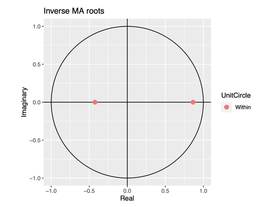
library(urca)
symbol0.ts %>% ur.kpss() %>% summary()
##
## #######################
## # KPSS Unit Root Test #
## #######################
##
## Test is of type: mu with 4 lags.
##
## Value of test-statistic is: 2.6058
##
## Critical value for a significance level of:
##                 10pct  5pct 2.5pct  1pct
## critical values 0.347 0.463  0.574 0.739
ndiffs(symbol0.ts)
## [1] 2
# for whole series, ndiffs() suggests second order differencing.
library(urca)
symbol0.ts[1:108] %>% ur.kpss() %>% summary()
##
## #######################
## # KPSS Unit Root Test #
## #######################
##
## Test is of type: mu with 4 lags.
##
## Value of test-statistic is: 2.1774
##
## Critical value for a significance level of:
##                 10pct  5pct 2.5pct  1pct
## critical values 0.347 0.463  0.574 0.739
ndiffs(symbol0.ts[1:108])
## [1] 1
# for whole series, ndiffs() suggests second order differencing.
symbol0.ts.arima<- auto.arima(symbol0.ts)
summary(symbol0.ts.arima)
## Series: symbol0.ts
## ARIMA(0,2,2)
##
## Coefficients:
library(urca)
##
##
## s.e.   0.0794   0.0795
##
## sigma^2 = 0.3385:  log likelihood = -123.02
## AIC=252.05   AICc=252.22   BIC=260.89
##
## Training set error measures:
##                      ME      RMSE       MAE         MPE      MAPE       MASE
## Training set 0.02149972 0.5736192 0.4093012 0.007226791 0.1626624 0.06733796
##                      ACF1
## Training set -0.007051954
autoplot(symbol0.ts.arima)
checkresiduals(symbol0.ts.arima)
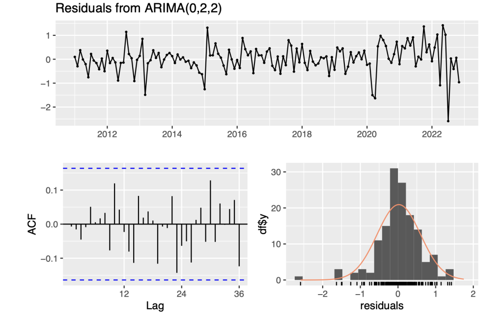
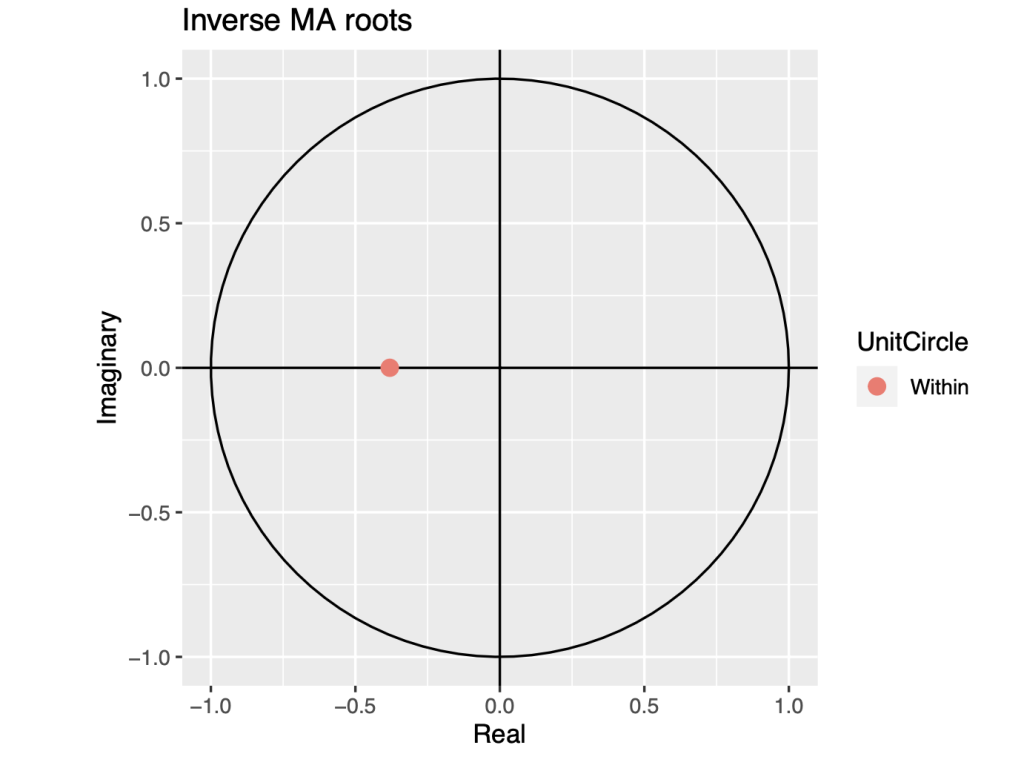
##
##  Ljung-Box test
##
## data:  Residuals from ARIMA(0,2,2)
## Q* = 16.696, df = 22, p-value = 0.7799
##
## Model df: 2.   Total lags used: 24
symbol0.ts.arima<- auto.arima(symbol0.ts[1:108])
summary(symbol0.ts.arima)
## Series: symbol0.ts[1:108]
## ARIMA(0,1,1) with drift
##
## Coefficients:
##          ma1   drift
##       0.3809  0.3518
## s.e.  0.0817  0.0567
##
## sigma^2 = 0.1854:  log likelihood = -60.6
## AIC=127.2   AICc=127.43   BIC=135.22
##
## Training set error measures:
##                      ME     RMSE       MAE          MPE      MAPE      MASE
## Training set 0.00159638 0.424554 0.3228736 0.0003542257 0.1355093 0.6720907
##                    ACF1
## Training set 0.03332243
autoplot(symbol0.ts.arima)
checkresiduals(symbol0.ts.arima)
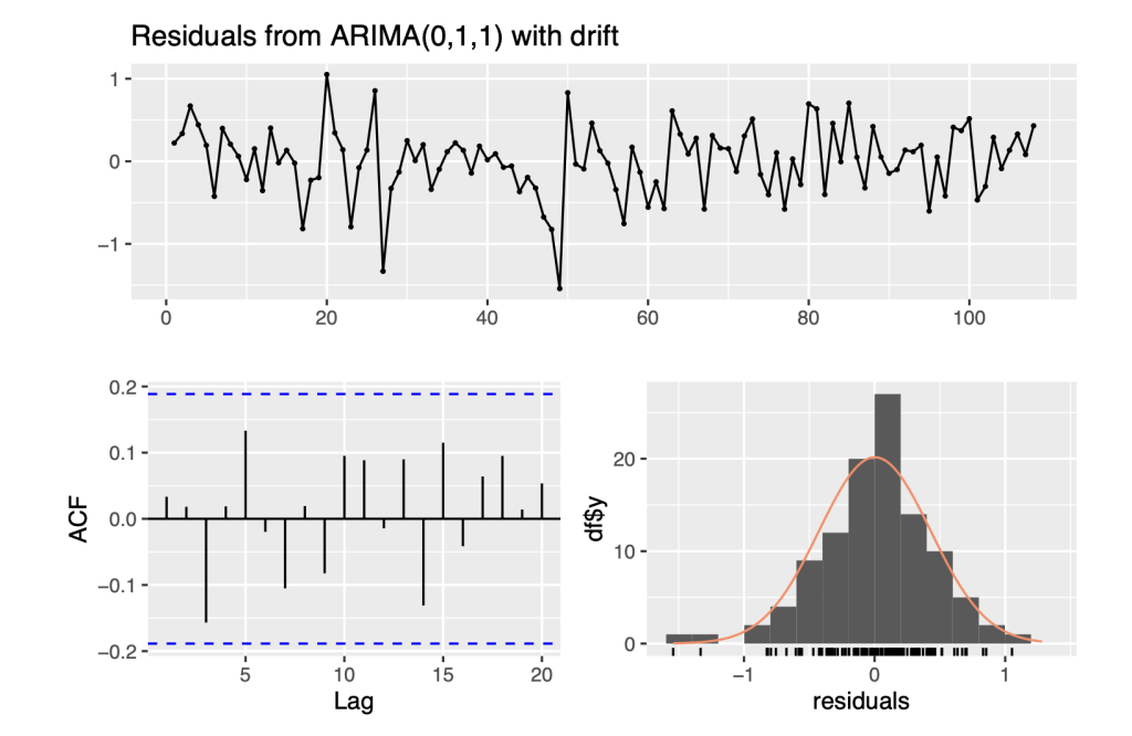
##
##  Ljung-Box test
##
## data:  Residuals from ARIMA(0,1,1) with drift
## Q* = 8.3315, df = 9, p-value = 0.5011
##
## Model df: 1.   Total lags used: 10
Based on the patterns observed in the data, we have determined that it follows an ARIMA(0,1,1) model. Two specific patterns in the data support this conclusion.
Firstly, the partial autocorrelation function (PACF) is either exponentially decaying or sinusoidal. This indicates that the data is dependent on its own past values and that the current value is related to the previous value with a certain degree of correlation. Secondly, there is a significant spike at lag 1 in the autocorrelation function (ACF), but none beyond lag 1. This implies that the data has a strong correlation with its immediate past value, but this correlation decreases rapidly as we move further away from the current value.
Overall, these observations suggest that the data has a certain degree of autocorrelation and season- ality, and that a time series model like ARIMA(0,1,1) would be appropriate to accurately capture these patterns and make meaningful predictions.
1.2.2 CPILFENS’s ARIMA Model :
Null hypothesis: The time series/ data is stationary.
We can use the R function auto.arima() to identify and specify a fitted auto-regressive integrated moving average (ARIMA) model.
In this case, the test statistic value is greater than the critical value at all levels of significance, which suggests that the symbol4.ts time series is non-stationary.
library(urca)
symbol4.ts %>% ur.kpss() %>% summary()
## # KPSS Unit Root Test #
## #######################
##
## Test is of type: mu with 4 lags.
##
## Value of test-statistic is: 2.8246
##
## Critical value for a significance level of:
##                 10pct  5pct 2.5pct  1pct
## critical values 0.347 0.463  0.574 0.739
ndiffs(symbol4.ts)
## [1] 2
# for whole series, ndiffs() suggests second order differencing.
library(urca)
symbol4.ts[1:108] %>% ur.kpss() %>% summary()
##
## #######################
## # KPSS Unit Root Test #
## #######################
##
## Test is of type: mu with 4 lags.
##
## Value of test-statistic is: 2.2526
##
## Critical value for a significance level of:
##                 10pct  5pct 2.5pct  1pct
## critical values 0.347 0.463  0.574 0.739
ndiffs(symbol4.ts[1:108])
## [1] 1
# for whole series, ndiffs() suggests second order differencing.
symbol4.ts.arima<- auto.arima(symbol4.ts)
summary(symbol4.ts.arima)
## Series: symbol4.ts
## ARIMA(2,2,2)(2,0,0)[12]
##
## Coefficients:
##          ar1      ar2      ma1     ma2    sar1    sar2
##       1.2534  -0.6942  -1.5742  0.7216  0.3195  0.3412
## s.e.  0.1310   0.0873   0.1515  0.1519  0.0848  0.0907
##
## sigma^2 = 0.1333:  log likelihood = -58.34
## AIC=130.68   AICc=131.52   BIC=151.32
##
## Training set error measures:
##                       ME      RMSE       MAE         MPE       MAPE       MASE
## Training set 0.002739018 0.3546955 0.2447811 0.001036818 0.09470889 0.03932631
##                    ACF1
## Training set 0.02117099
autoplot(symbol4.ts.arima)
checkresiduals(symbol4.ts.arima)
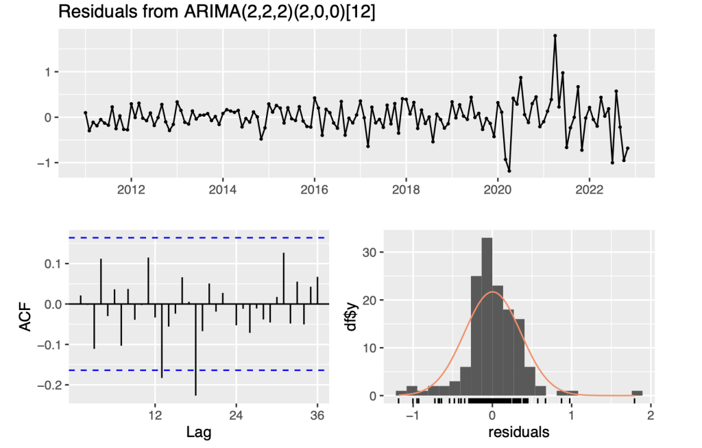
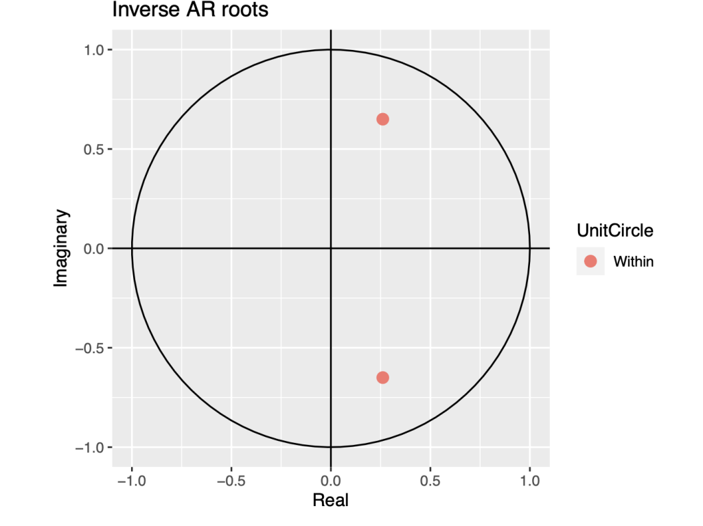
##  Ljung-Box test
##
## data:  Residuals from ARIMA(2,2,2)(2,0,0)[12]
## Q* = 25.447, df = 18, p-value = 0.1131
##
## Model df: 6.   Total lags used: 24
symbol4.ts.arima<- auto.arima(symbol4.ts[1:108])
summary(symbol4.ts.arima)
## Series: symbol4.ts[1:108]
## ARIMA(2,1,0) with drift
##
## Coefficients:
##          ar1      ar2   drift
##       0.5217  -0.4906  0.3999
## s.e.  0.0853   0.0850  0.0279
##
## sigma^2 = 0.08015:  log likelihood = -15.3
## AIC=38.6   AICc=38.99   BIC=49.29
##
## Training set error measures:
##                       ME     RMSE       MAE         MPE       MAPE      MASE
## Training set 0.002997304 0.277811 0.2278571 0.001007415 0.09316369 0.5187606
##                     ACF1
## Training set -0.02481104

autoplot(symbol4.ts.arima)
checkresiduals(symbol4.ts.arima)
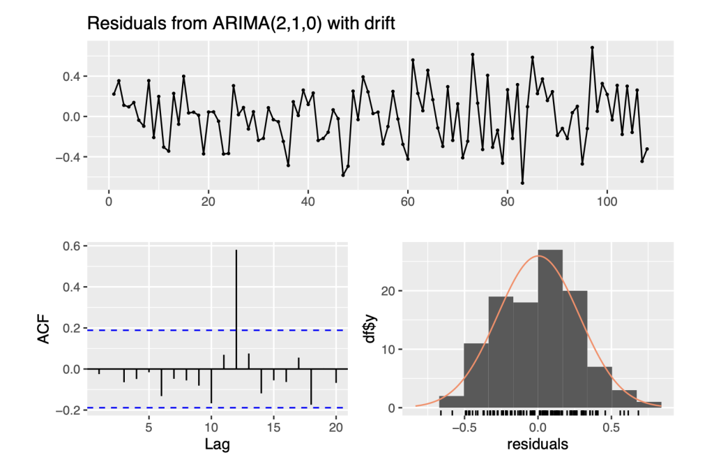
##
##  Ljung-Box test
##
## data:  Residuals from ARIMA(2,1,0) with drift
## Q* = 7.6742, df = 8, p-value = 0.4659
##
## Model df: 2.   Total lags used: 10
So, ARIMA(2,1,0) with drift means that the model has an autoregressive component of order 2, a degree of differencing of 1, no moving average component, and a constant term. The AR and MA components capture the autocorrelation and moving average patterns in the data, respectively, while the drift term captures the overall trend or level of the data. The drift term in the ARIMA model suggests that there may be a trend or a systematic change in the mean of the data over time that is not explained by the AR or MA components.
The ACF plot shows one line crossing the blue critical lines between the lags of 10 and 15, then it suggests that there is some significant autocorrelation still present in the residuals of the model. This means that the model may not be fully capturing all the relevant information in the data. It may be necessary to either modify the existing model or try alternative approaches to improve the fit.
1.3 Discussion of ARIMA models based on the coefficients obtained
1. Coefficient Table for CPILFENS Model – ARIMA(2,1,0) with Drift :
Coefficient Estimate Standard Error AR1 0.5217 0.0853 AR2 -0.4906 0.0850 Drift 0.3999 0.0279
2. Coefficient Table for CPIAUCSL Model – ARIMA(0,1,1) with drift :
Coefficient Estimate Standard Error MA1 0.3809 0.0817 Drift 0.3518 0.0567
3. Coefficient Table for CPILFESL Model – ARIMA(1,2,1) :
Coefficient Estimate Standard Error AR1 0.1956 0.1014 MA1 -0.9525 0.0344
Interpreting these parameter estimates can offer valuable insights into the underlying dynamics of the time series. For instance, positive autoregressive (AR) parameters often correspond to momentum or persistence in the series. This implies that the series tends to continue moving in the same direction as its past values. On the other hand, negative AR parameters suggest mean reversion, indicating that the series tends to revert back towards its mean over time.
Additionally, positive moving average (MA) parameters indicate that recent forecast errors have a momentum-like effect on the series. This means that deviations from the forecast tend to be corrected over subsequent time periods. Such insights obtained from the parameter estimates provide a deeper understanding of the time series data.
About the author

Ruthvik Reddy Bommireddy
Ruthvik is a 12th grade student at the Delhi Public School Bangalore North, India. His academic focus lies at the intersection of Science and Economics, driven by a desire to create positive change in the world through future ventures. Ruthvik enjoys basketball, tennis, and roller skating, as well as drawing and sketching. He also serves as the president and founder of his school’s business club.