

Author: Avi Shukla
Mentor: Dr. Osman Yağan
Leland High School
Abstract
Imagine being given several slot machines [bandits], each rigged to provide a variable amount of money, and are asked to play a total of T times across all machines. The problem leaves one in a puzzling dilemma as people naturally want to test every available option to confidently secure the best bandit. However, people do not wish to lose potential profit by employing substandard bandits. This fundamental trade-off of exploration vs. exploitation is the essence of a widely relevant issue we dub the “multi-arm bandit problem.” Multi-armed bandits are powerful and dynamic algorithms used to make decisions under uncertainty. Bandits come in a wide variety and assortment of which one would pick based on their situation and desired approach. Throughout this paper, we will explore the various algorithms one can utilize to address the multi-arm bandit problem and any potential benefits and drawbacks of each method. This paper will discuss the evolution of multiple bandit methods and algorithms in a simple, digestible, and educational format.
Keywords: Bandit, Multi-armed bandits, Stochastic Bandits, explore then commit, ETC, Upper Confidence Bound, UCB, UCB Minimax Optimality, MOSS, Adversarial Bandits, Contextual Bandits, machine learning
Introduction
A bandit problem is a sequential game played between the learner and the environment over many rounds. The positive natural number n, termed the horizon, denotes the number of rounds that will be played. The learner’s goal is to maximize cumulative rewards within the set horizon. The challenge comes from how the environment is hidden from the learner, forcing them to use their histories created from their previous actions. The learner can map these histories to efforts to develop a policy that can guide a learner’s interactions through an environment.
To gauge the quality of our predictions, we can utilize regret, where we measure the learner’s performance with the optimal competitor class policy, obtaining tangible feedback about the learner. The main goal is simply to minimize regret as much as possible over all possible environments, resulting in a policy nearly identical to one of the environment classes. Whereas regret is for an individual trial t, we can also measure the mean difference between the best arm and an arm “i” through the sub-optimality gap often represented with ∆.
As per regret theory, the optimization problem for the decision-maker is usually to minimize regret, which is different from maximizing utility. One strange aspect of this measure of “regret” is that it can be negative (i.e., you can gain more than expected). Hence, this measure of “regret” does not correspond to the usual definition in regret theory nor the expected regret in regret theory. It is a hybrid of these and does not obey the property of non-negativity.
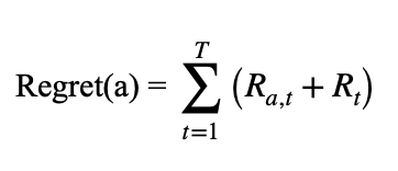
Let Ra,t denote the return at time t for action a = 1,….K
Let a = (a1,….at) denote the vector of actions, and
Let Rt = Ra,t denote the return of the chosen action at the time t
then the usual form for regret would be the random variable:
There is a multitude of bandit algorithms, some of which are described below.
Stochastic bandits are generally defined with the rewards for each specific arm independently and identically distributed from a probability distribution. Different Stochastic Bandits algorithms are explored below.
Explore then Commit Algorithm (ETC)
One of the simplest kinds of stochastic bandit algorithms is dubbed the “explore then commit” algorithm (ETC), also sometimes known as the greedy algorithm. The algorithm explores a total of “m” (times explored each arm) × k (number of arms) times before committing to an arm. The formal equation is as follows:
- At = (t mod k) + 1, if t At = (t mod k) + 1 , if t ≤ mk ; or
- At = argmaxi μ^i(mk), if t > mk
It is important to note that if “m” becomes too large, the policy explores for longer than it should, whereas if “m” is too tiny, the probability the algorithm commits to the wrong arm will grow. Therefore, choosing “m” becomes integral to the algorithm’s performance. Choosing m, in turn, becomes one of the algorithm’s most significant drawbacks as it tends to be chosen blindly. Moreover, due to the non-adaptive nature of “m,” optimizing it to select a good constraint can become challenging.
A massive benefit to ETC is the ease and practicality at which one can work with them, making them ideal candidates for a simple algorithm to get the job done. ETC generally behaves best with two arms (also known as A/B testing) but loses effectiveness as more arms are added. Another issue is that the algorithm is not at anytime; i.e., it requires knowing the horizon “n.” However, this limitation can generally be overcome by utilizing a method known as the doubling trick, allowing the algorithm to develop and polish itself without being halted by the horizon.
The Optimistic-Greedy Algorithm
A simple way to modify the Greedy Algorithm, to make it explore the set of available actions in search of the optimal action, is to set the initial action estimates to very high values.
By allowing exploration time “m” to become a data-dependent variable, it is possible to heavily optimize the regret without knowledge of the sub-optimality gap. This method is known as successive elimination and works with increasingly sensitive hypothesis tests, which slowly eliminate arms. Specifically, it alternates arms until “a” is worse than some other arm with a high probability, subsequently discarding arm “a” and narrowing the selection of arms.
The major drawback of the Optimistic-Greedy algorithm is that a poorly chosen initial value can result in a sub-optimal total return. Selecting the best initial deals can be challenging without prior knowledge of the range of possible rewards.
The Epsilon-Greedy Algorithm (ε-Greedy)
A pure Greedy strategy has a very high risk of selecting a sub-optimal hand and sticking with it.
ETC algorithms also have a randomized relative known as the ε-Greedy algorithm. At round “t”, the algorithm either plays the empirically best arm with the probability “1-εt” or simply explores. The Epsilon-Greedy strategy is an easy way to add exploration to the basic Greedy algorithm. Due to the random sampling of actions, the estimated reward values of all actions will converge on their valid values.
The downside of the ε-Greedy algorithm is that non-optimal actions continue to be chosen, and their reward estimates are refined long after they have been identified as non-optimal.
The Upper Confidence Bound (UCB) Algorithm
The ETC algorithm and its variations do not fare well for a generic solution. The pure Greedy algorithm does not fare much better than a simple random selection method. However, with some slight modifications, such as Optimistic-Greedy’s use of large initial values or Epsilon Greedy’s approach of introducing random exploration, the selection performance can be significantly improved. Optimistic-Greedy’s performance depends on the values selected for its initial rewards. Epsilon Greedy continues to explore the set of all actions long after it has gained sufficient knowledge to know which actions are insufficient.
To improve the performance, what if we could take ETC but make the algorithm more dynamic? The answer to this question comes with a new algorithm known as Upper confidence Bound Bandit or UCB. This algorithm is called UCB, as we are only concerned with the upper bound, given that we are trying to find the arm with the highest reward rate. UCB has several advantages over ETC as it does not depend on advanced knowledge of the sub-optimality gap, behaves well with more than two arms, and depends on the horizon “n,” which can also be eliminated with the aforementioned doubling trick.
The unknown mean of the ith arm can be defined as
- UCBi(t − 1, δ) = ∞ if Ti( t – 1 ) = 0; if Ti( t – 1 ) = 0
- UCBi(t − 1, δ) = μi( t – 1 ) + √(2 log(1/δ) / Ti(t−1)); otherwise
Where δ is the confidence level, μ is the mean subgaussian random variable, and t is the round number where the learner has observer Ti (t-1) samples from arm i and received rewards from that arm with an empirical mean of μi( t – 1 ).
Something to note about UCB is that it functions on the principle of optimism under uncertainty, which states that one should act as if the environment is as nice as possible. It achieves optimism by adding the exploration bonus √(2 log(1/δ) / Ti(t−1)), which, unlike ETC, allows underrepresented arms to be favored so they don’t fall behind.
The algorithm for UCB(δ) can be given as
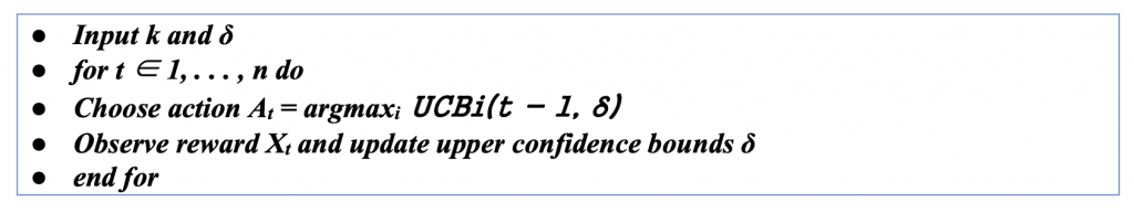
UCB functions as an index algorithm, meaning it tries to maximize a quality metric called the index which can be used to compare rewards from different arms. In the case of UCB, this index is the sum of the empirical mean of the rewards experienced in conjugation with the aforementioned exploration bonus, also called confidence width.
Note that choosing the correct value of confidence level “δ” is not easy. It needs to balance to ensure optimism with high probability but still deter suboptimal arms from being explored excessively.
If ETC is tuned with the optimal choice of commitment time for each choice ∆, it can outperform the parameter-free UCB; otherwise, it will not outperform UCB. We will explore a variant of UCB which will outperform the ETC with even optimally tuned ETC.
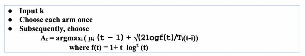
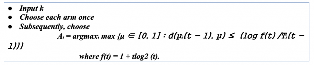
UCB Algorithm: Asymptotic Optimality
This algorithm is asymptotically optimal, meaning that no algorithm can perform better than it in the limit of horizon n going to infinity. Put differently, if the algorithm is to be used for a long time, then the algorithm presented next is optimal. In the UCB described earlier, the right confidence level “δ” value is not easy, and if not chosen optimally, the results are suboptimal. Asymptotically optimal UCB can be described by
Regret bound for the above algorithm is much more complicated than choosing the static value for the UCB algorithm. The important thing is that the dominant terms have the same order, but the constant multiplying the dominant term is smaller. The significance of this is that the long- term behavior of the algorithm is controlled by this constant. The worst-case regret for the above algorithm is
- Rn = O(√(kn log(n))
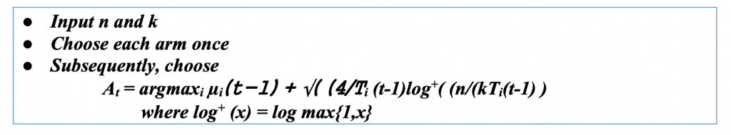
UCB Algorithm: Minimax Optimality (MOSS)
The UCB Minimax Optimality (MOSS) algorithm is an asymptotically optimal algorithm. The worst-case regret for the above algorithm is Rn = O(√(kn log(n)). By modifying the confidence levels of the algorithm, it is possible to remove the log factor entirely. Building on UCB, the directly named ‘minimax optimal strategy in the stochastic case’ (MOSS) algorithm was the first to make this modification, as presented below. MOSS again depends on prior knowledge of the horizon, a requirement that may be relaxed, as we explain in the notes. The term minimax is used because, except for constant factors, the worst-case bound proven in this chapter cannot be improved on by any algorithm.
One of these algorithms’ main novelties is how their confidence level can be chosen based on the number of plays for individual arms, as well as for “n” and “k.” The significance of this algorithm is that, unlike UCB, it tries to optimize the worst-case regret.
The USB MOSS algorithm can be given as the following algorithm.
While being nearly asymptotically optimal is a huge advantage, the algorithm also has two significant drawbacks. Asymptotic regret often leads to a finite time regret, meaning that for a shorter horizon, the algorithm would perform worse than UCB but would converge to match as the horizon moves toward infinity. Another issue lies with the algorithm that pushes the expected regret to be lowered too hard, causing the distribution of regret to be unstable and much less well-behaved.
UCB: Bernoulli Noise (KL-UCB)
In previous algorithms, we assumed that the noise of the rewards was σ-subgaussian for some known σ > 0. This has the advantage of simplicity and relative generality, but stronger assumptions are sometimes justified and often lead to more robust results. Suppose the rewards are assumed to be Bernoulli, which means that Xt ∈ {0, 1}. This is a fundamental setting found in many applications. For example, in click-through prediction, the user either clicks on the link or not. A Bernoulli bandit is characterized by the mean pay-off vector μ ∈ [0, 1]k and the reward observed in round t is Xt ∼ B(μAt ).
The difference between KL-UCB and UCB is that bounds are used to define the upper confidence bound. The algorithm is given as follows:
This algorithm works best when there are only two choices [0,1] or closes to 0 or 1. It could be used for many practical applications which need a binary selection; as the number of choices increases in range, it becomes more and more undesirable.
Adversarial Bandits
Adversarial bandits force the user to drop all preexisting notions of how rewards are generated except that they are in a bounded set and are chosen without knowing the learner’s actions. This forces us to redefine our existing idea of regret from being worse than an optimal policy to simply being worse than a set of constant policies. Unlike stochastic bandits, there is nothing to be learned from as we cannot now assume there is a fixed distribution or that there is any specific rule to how it changes. While harder to work with, the benefit of such a setting is that algorithms will generally be more robust than their stochastic counterpart.
Adversarial Bandits – The Exp3 Algorithm
The EXPonential weight algorithm for EXPloration and EXPloitation (EXP3) is one such algorithm that functions in the adversarial setting. The EXP3 algorithm functions by utilizing exponential weighting, where it maintains a set of weights for each action to decide the next step randomly. Based on whether the resulting payoff is good or bad, these weights will either increase or decrease in value. The formal equations are as follows:

It is important to note that η is the learning rate. When the learning rate is large, Pt concentrates on the arm with the most significant estimated reward, and the algorithm exploits aggressively. As Pt focuses, it causes the variance of weights for poorly performing arms to increase dramatically, making it an unreliable estimator. Conversely, Pt is more uniform for small learning rates, and the algorithm explores more frequently.
Adversarial Bandits – The Exp3-IX Algorithm
The objective of EXP3-IX is to modify EXP3 so that the regret stays small in expectation and is simultaneously well concentrated about its mean. Such results are called high-probability bounds. The poor behavior of EXP3 occurs because the variance of the importance-weighted estimators can become very large.
EXP3-IX, where IX stands for implicit exploration, adds a chosen constant γ to the divisor to smoothen the variance and hence a better estimator. γ could be constant or calculated after each arm.
Contextual Bandits
The algorithms introduced so far work well in stationary environments with only a few actions. Unfortunately, real-world problems are seldom this simple. For example, a bandit algorithm designed for targeted advertising may have thousands of actions. Even more troubling, the algorithm can access contextual information about the user and the advertisement. Ignoring this information would make the problem highly non-stationary, but the earlier algorithm cannot use these contexts.
While everything previously discussed can be helpful, when moving into the algorithms implemented into real-life scenarios, many more external factors termed “contexts” were previously not present. This is additional information that may help predict the quality of action. When including contexts in the algorithms, we bias our regret to align with the expert opinion. This context weight for each arm can dynamically change with the determination of each trial.
These contexts can directly influence any of the algorithms discussed earlier to get better results. It is vital to have the proper context. Else, we may end up getting the wrong conclusions. For example, if somebody is trying to choose a movie rating from Russia, we can conclude that they would prefer a Russian movie, and we can give higher weight to Russian-language movies. But an American traveling to Russia might get recommendations for Russian-language movies unless we keep the contexts that he is American, which overweighs the other recommendation.
Contextual Bandits – Bandits with Expert Advice
When the context set C is extensive, using one bandit algorithm per context will almost always be a poor choice because the additional precision is wasted unless the amount of data is enormous. Fortunately, however, it is seldom the case that the context set is both large and unstructured.
For example, the person’s demographics might reduce the bigger set into the smaller set to get better rewards. This could be done on the smaller partition of arms and use a similarity function for better predictions. Yet another option is to run a supervised learning method, training on a batch of data to find better predictions.
Contextual Bandits – Exp4
The number “4” in Exp4 is not just an increased version number, but rather indicates the four e’s in the official name of the algorithm (exponential weighting for exploration and exploitation with experts). The idea of the algorithm is straightforward. Since exponential weighting worked so well in the standard bandit problem, we aim to adapt it to the problem at hand. However, since the goal is to compete with the best expert in hindsight, it is not the actions we will score but the experts. Exp4 thus maintains a probability distribution Qt over experts and uses this to come up with the following action in an obvious way, by first choosing an expert Mt at random from Qt and then following the chosen expert’s advice to select At ∼ E (t) Mt. This is the same as sampling At from Pt = QtE(t) where Qt is treated as a row vector. Once the action is chosen, one can use their favorite reward estimation procedure to estimate the rewards for all the actions. This is then used to estimate how much total reward the individual experts would have made so far. The reward estimates are then used to update Qt using exponential weighting.
Real Life Uses
Bandit algorithms have a wide variety of use cases. One of the most basic ways it is applied is through A/B testing, which functions like the ETC algorithm but with only two arms. Another common application of bandits can be routing the best path, whether from network routing to routing in transportation systems. Another common application is dynamic pricing, where a bandit algorithm can adjust prices by classifying them as either “too high” or “too low” until it finds an optimal price range.
Contextual bandit algorithms are commonly utilized in advert placement, where contexts are used to decide what a user is interested in. An example of context can be when a user recently searched for pet food; one might want to recommend pet-based items. This kind of advertising based directly on a user’s history is known as targeted advertising in the marketing world and is a common practice by many companies. However, it is essential to understand that finding the best result is not as simple as “choose an algorithm and use it” as with real-world problems like advertising. Real-world scenarios involve many more essential things than maximum clicks, such as freshness, fairness, and satisfaction, to name a few. These extra factors can make it challenging to implement bandits into the real world as they will often require lots of extra work to overcome. Another common usage of contextual bandit algorithms can be seen in recommendation systems, commonly used by companies like Netflix for personalized recommendations. For recommendation systems with companies like Netflix in particular, building a recommendation system can be challenging as the set of all arms is extremely large, and the movies the user picks to watch are relatively few. The reward for a movie will typically be calculated by combining (1) the movie watch time and (2) the movie rating. This kind of reward measurement can lead to another problem where the algorithm will recommend only certain movies. Therefore, only those specific movies will have any data, while those with no data are left out of the loop. There are always ways around this, such as putting a “new/upcoming series” to promote shows and movies with fewer data. It is essential to understand that implementing a contextual bandit algorithm for the real world requires much more consideration and creative usage than stochastic bandits, as the problems faced are inherently more complex and multi-layered. Below are provided links to examples of places bandit algorithms can be found.
- Google Analytics
- Washington Post
- Netflix presentation on their bandit algorithms
- Network routing with BGP
- StitchFix Experimentation Platform
Conclusion
Multi-armed bandits have been studied for over a century. New and more robust algorithms are constantly introduced, typically as combinations of the algorithms discussed here or their variations. Naturally, practical applications are combination algorithms for more reinforcement learning. None of the above algorithms are suited to all applications, and careful consideration of specific applications and the data available is needed to decide which algorithm best fits your use. For any further research, one can turn to GitHub, as it contains many implementations of the algorithms discussed in this paper.
References
Lattimore, Tor, and Szepesv ́ari, Csaba, Bandit Algorithms (1st edition), Cambridge University Press (
Slivkins, Aleksandrs: Introduction to Multi-Armed Bandits, Foundations and Trends in Machine Learning (2019)
Sutton, R.S., Barto, A.G.: Reinforcement Learning: An Introduction. MIT Press, Cambridge, MA (1998)
Watkins, C.: Learning from Delayed Rewards. Ph.D. thesis, University of Cambridge, Cambridge, England (1989)
Zhao, Qing, and Srikant, R.: Multi-Armed Bandits: Theory and Applications to Online Learning in Networks (Synthesis Lectures on Communication Networks) (2019)
About the author
Avi Shukla
Avi is a senior at Leland High School, San Jose, CA. He is interested in Data Science, machine learning, and artificial intelligence. Avi is fascinated by how neural networks can emulate the thinking and learning process of the human mind. He loves reading all kinds of books, and his current interests include reading and learning human psychology. Avi has been trained in classical piano since childhood and loves arranging music. He loves to go on long biking trips and hikes whenever possible.