Time Series Modelling of India Consumer Price Index

Abstract

In this paper, we develop a time series model for forecasting the India Consumer Price Index (CPI). The time series begins in the month of January, in the year 1960. The frequency of the time series is based on a monthly pattern. The original time series is non stationary based on the results of a few tests. To resolve the issue of non stationarity, the time series is transformed to the logarithm scale. Ordinary and seasonal differences are applied to the time series to remove non stationarity. Unit root tests such as ADF and KPSS tests are applied to the transforms of the original time series. These tests help prove if the transforms of the series are consistent with being stationary. Different forecasting methods are applied to the time series to forecast a 12 month period following the end of the time series.

1. Introduction

The aim of this paper is to understand the concept of time series and implement forecasting methods on time series using R Studio.

A Consumer Price Index (CPI) is designed to measure the changes over time in general level of retail prices of selected goods and services that households purchase for the purpose of consumption. Such changes affect the real purchasing power of consumers’ income and their welfare. The CPI measures price changes by comparing, through time, the cost of a fixed basket of commodities. [1]

Given below is a basic outline of the paper, section-wise:

• Section 2 : In this section, the time series is displayed and basic analysis functions are performed on the time series.
• Section 3 : Naive forecasting method is implemented on the time series.
• Section 4 : Logarithm transform is performed on the time series and forecasting methods are imple- mented on the transformed time series.
• Section 5 : Unit root tests are applied on the time series to determine the stationarity of the series. Dif- ferencing methods are performed on the time series to convert non-stationary time series to stationary time series.
• Section 6 : Forecasting methods such as ARIMA model is implemented on the time series and further analysis is done.

2. R Analysis: Setup

2.1 Load libraries

Load all the necessary libraries to perform the required functions on R Studio.

library(tidyverse) 

## — Attaching packages ————————————— tidyverse 1.3.2 —
## v ggplot2 3.3.6 v purrr 0.3.4 ## v tibble 3.1.8 v dplyr 1.0.10
## v tidyr 1.2.0 v stringr 1.4.1
## v readr 2.1.2 v forcats 0.5.2
## — Conflicts —————————————— tidyverse_conflicts() —
## x dplyr::filter() masks stats::filter()
## x dplyr::lag() masks stats::lag()

library(tidyquant)

## Loading required package: lubridate ## ## Attaching package: ’lubridate’
##
## The following objects are masked from ’package:base’:
##
## date, intersect, setdiff, union
##
## Loading required package: PerformanceAnalytics
## Loading required package: xts
## Loading required package: zoo
##
## Attaching package: ’zoo’
##
## The following objects are masked from ’package:base’:
##
## as.Date, as.Date.numeric
##
##
## Attaching package: ’xts’
##
## The following objects are masked from ’package:dplyr’:
##
## first, last
##
##
## Attaching package: ’PerformanceAnalytics’
##
## The following object is masked from ’package:graphics’:
##
## legend
##
## Loading required package: quantmod
## Loading required package: TTR
## Registered S3 method overwritten by ’quantmod’:
##   method from
##   as.zoo.data.frame zoo

library(fpp2) 

## — Attaching packages ———————————————- fpp2 2.4 —
## v forecast 8.17.0 v expsmooth 2.3
## v fma 2.4

library(readr) 
library(tseries) 
library(forecast) 
library(Metrics)

##
## Attaching package: ’Metrics’
##
## The following object is masked from ’package:forecast’:
##
## accuracy

2.2 Import data

Load the data set into a variable and change the format of the ‘Date’ column. The data is stored in a variable named ‘INDCPIALLMINMEI’. The reference for this data set is:

• “Organization for Economic Co-operation and Development, Consumer Price Index: All Items for India [INDCPIALLMINMEI], retrieved from FRED, Federal Reserve Bank of St. Louis; https://fred. stlouisfed.org/series/INDCPIALLMINMEI, November 22, 2022.”

INDCPIALLMINMEI <- read_csv("INDCPIALLMINMEI.csv",
col_types = cols(DATE = col_date(format = "%Y-%m-%d")))

2.3 Plot time series

The data stored in variable ‘INDCPIALLMINMEI’ is converted into a time series and stored in the variable ‘Y’. The time series starts from January of 1960. The ‘Frequency’ parameter is set to 12. This indicates that the data is spanned for each month of the year. The time series ends in the month of July, in the year 2022.

Y <- ts(INDCPIALLMINMEI$INDCPIALLMINMEI, start = c(1960,1), frequency = 12)
autoplot(Y) + labs(title = "CPI of India") + xlab("Year") + ylab("CPI")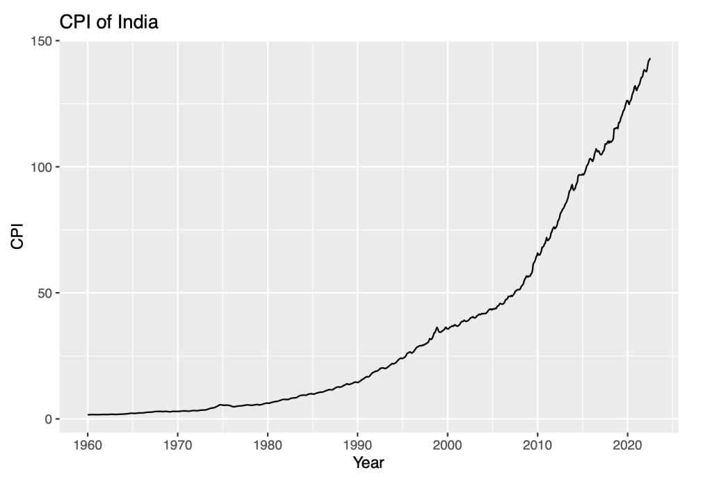

2.4 Apply Decompose function

Decompose a time series into seasonal, trend and irregular components using moving averages. Deals with additive or multiplicative seasonal component. The components of decompose function are as follows:

• Data: Plots the values of a time series.
• Trend: Pattern in time series that depicts the local movement of a series over time. A trend can be upwards or downwards depending on the data and the local period of time.
• Seasonality: The data repeats itself in a periodic manner regularly over a period of time.
• Remainder: The part of the time series that is left after removing the trend and seasonal components. It is the random fluctuations in the time series that the trend and seasonal components cannot explain.

autoplot(decompose(Y))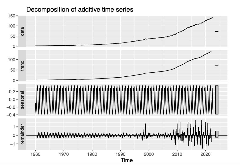

From the above figure, we can see that there is a gradual upward trend in the time series. Seasonal component is present. The values in the remainder series increases with time. The remainder series resembles white noise prior to 1996. After 1996, there is an increase in variance through the end of the series. This pattern suggests that the residual time series is non-stationary. We can test if the time series is non-stationary. We perform a few tests on the time series to produce a definitive answer on stationarity or non-stationarity.

3. Analysis of Time series

3.1 ACF and PACF

Using Autocorrelation analysis, we are able to detect patterns and check for randomness in time series.

Autocorrelation Function (ACF) is a statistical technique that we can use to identify how correlated the values in a time series are with each other. The ACF plots the correlation coefficient against the lag, which is measured in terms of a number of periods or units. The gap between two measurements is known as ‘lag’. The values are plotted along with the confidence interval in ACF. ACF finds the how the present value of the original time series is related to it’s lagged or past values. ACF considers all the time series components such as trend, seasonality, cyclic and residual while finding the correlations.

Partial Autocorrelation Function (PACF) determines the correlation of the residuals with the next lag value. Residual are the remaining part after removing the the effects. If there is any hidden information from the residual, we can get a good correlation if the residual is modelled by the next lag. The next lag is kept as the feature while modelling.

ggAcf(Y)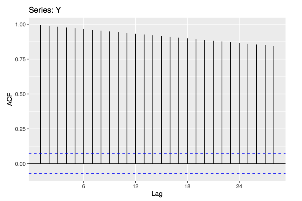

ggPacf(Y)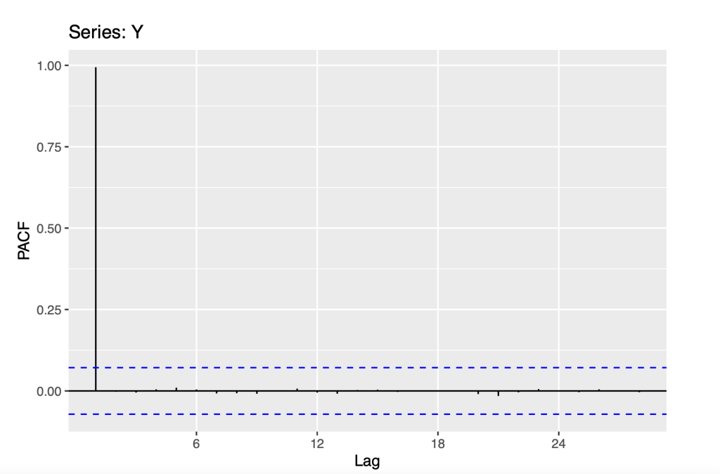

As seen from the ACF Plot, there is an exponential decrease. The exponential decrease is consistent with the non stationarity that may be a random walk. The PACF plot shows us that only the first lag auto correlation is statistically significant, which is also consistent with a random walk model.

In the next couple of sections, we apply the naive forecast method and random walk model with drift. This will help us identify an appropriate model. In each case, we report the fitted model statistics, check the residuals for consistency with white noise and illustrate forecasts of the fitted model.

3.2 Naive forecasting model of the original series

The Naive forecasting method is one the simplest forecasting method. This method takes into account the most recent observation to forecast the next observation. The forecast in the upcoming period is equal to the value observed in the previous period. The Naive forecasting method is specified with the R function ‘naive’.

Y_naive <- naive(Y) 
print(summary(Y_naive))

##
## Forecast method: Naive method
##
## Model Information:
## Call: naive(y = Y)
##
## Residual sd: 0.4625
##
## Error measures:
## ME RMSE MAE MPE MAPE MASE
## Training set 0.1885862 0.4625323 0.2589692 0.5864412 0.867108 0.1152025
## ACF1
## Training set 0.394911
##
## Forecasts:
## Point Forecast Lo 80 Hi 80 Lo 95 Hi 95
## Aug 2022 143.1186 142.5259 143.7114 142.2121 144.0252
## Sep 2022 143.1186 142.2803 143.9569 141.8366 144.4007
## Oct 2022 143.1186 142.0919 144.1453 141.5484 144.6888
## Nov 2022 143.1186 141.9331 144.3041 141.3055 144.9317
## Dec 2022 143.1186 141.7932 144.4441 141.0915 145.1457
## Jan 2023 143.1186 141.6667 144.5706 140.8981 145.3392
## Feb 2023 143.1186 141.5503 144.6869 140.7201 145.5171
## Mar 2023 143.1186 141.4421 144.7952 140.5545 145.6827
## Apr 2023 143.1186 141.3404 144.8969 140.3990 145.8383
## May 2023 143.1186 141.2442 144.9931 140.2519 145.9854

checkresiduals(Y_naive)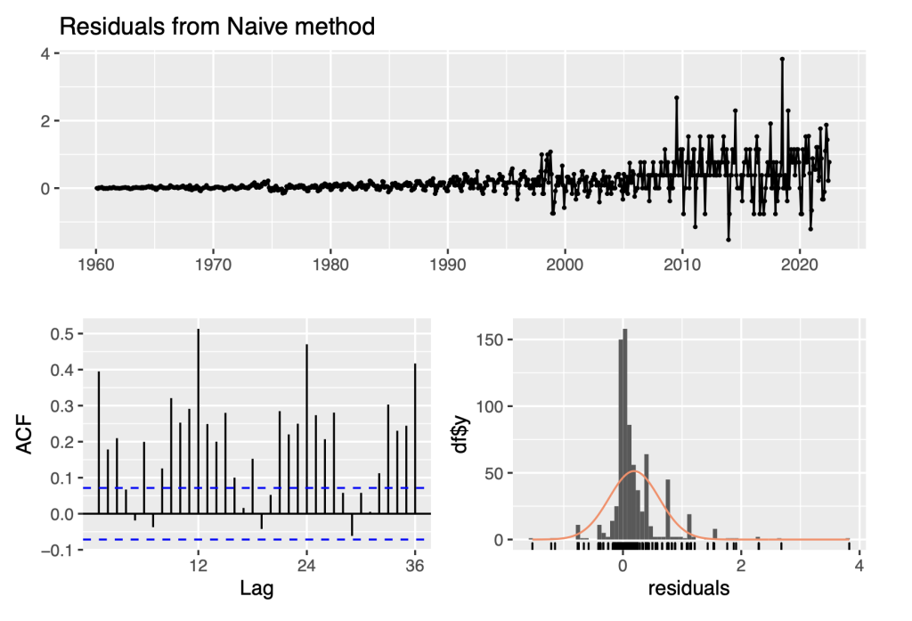

##
## Ljung-Box test
##
## data: Residuals from Naive method
## Q* = 1102.6, df = 24, p-value < 2.2e-16
##
## Model df: 0. Total lags used: 24

f12 = forecast(Y_naive)
autoplot(f12, include = 60)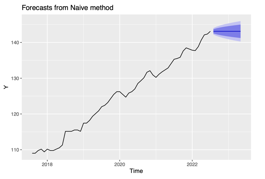

It is apparent that the residuals for the naive model are definitely not consistent with being white noise, because their variability increases over time. To resolve this issue, we transform the series to the logarithm scale and repeat the same analysis as before.

4. Analysis of the Logarithm Transform of the Time Series

From Section 3, it is apparent that the residuals for the naive model are definitely not white noise, because their variability increases over time. To resolve this issue we transform the series to the logarithm scale and repeat the same analysis as before.

4.1 ACF and PACF

Again, we use Autocorrelation analysis, to detect patterns and check for randomness in the logarithm trans- form of the time series.

Ylog=log10(Y)
ggAcf(Ylog)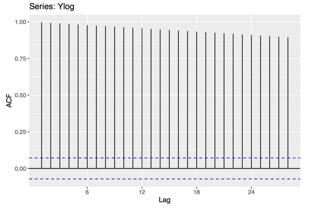

ggPacf(Ylog)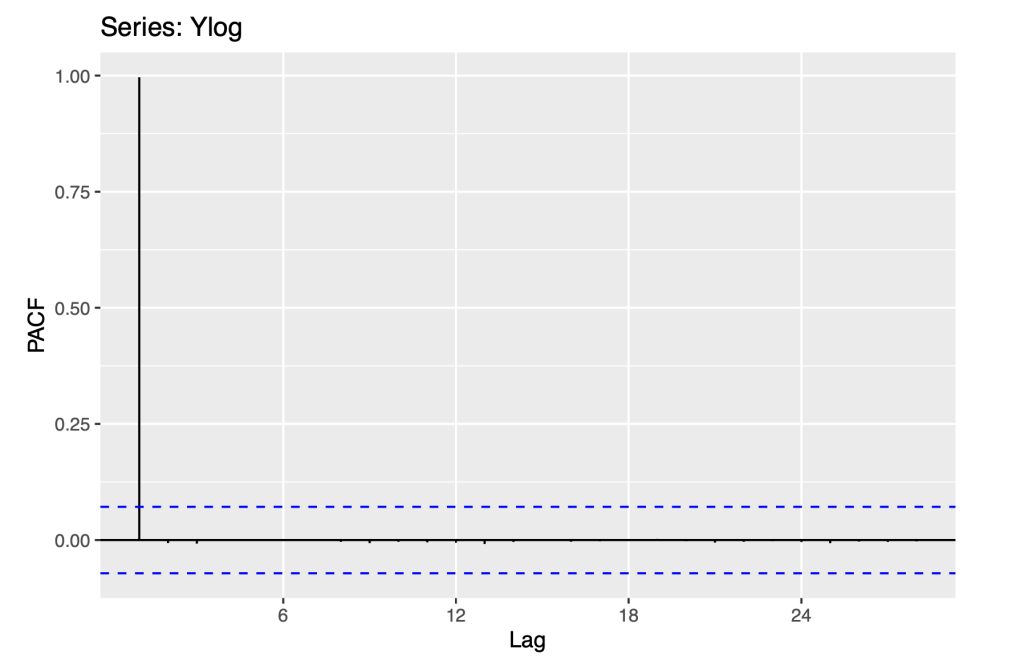

There is an exponential decrease that is seen in the ACF plot. The first order auto correlation is statistically significant, which is also consistent with a random walk. The above ACF and PACF plot are similar to the observations from section 3.1 .

4.2 Naive Forecasting of the Logarithm transform

The Naive forecasting method is performed on the logarithm transform time series. This gives us an indication of how the time series has changed with respect to the original time series.

Ylog_naive <- naive(Ylog)
print(summary(Ylog_naive))

##
## Forecast method: Naive method
##
## Model Information:
## Call: naive(y = Ylog)
##
## Residual sd: 0.0049
##
## Error measures:
## ME RMSE MAE MPE MAPE MASE
## Training set 0.002574199 0.004883262 0.003785647 0.2983802 0.4735897 0.1159322
## ACF1
## Training set 0.4691113
##
## Forecasts:
## Point Forecast Lo 80 Hi 80 Lo 95 Hi 95
## Aug 2022 2.155696 2.149438 2.161954 2.146125 2.165267
## Sep 2022 2.155696 2.146846 2.164547 2.142161 2.169232
## Oct 2022 2.155696 2.144857 2.166536 2.139119 2.172274
## Nov 2022 2.155696 2.143180 2.168212 2.136554 2.174838
## Dec 2022 2.155696 2.141703 2.169690 2.134295 2.177098
## Jan 2023 2.155696 2.140367 2.171025 2.132252 2.179140
## Feb 2023 2.155696 2.139139 2.172254 2.130374 2.181019
## Mar 2023 2.155696 2.137995 2.173397 2.128625 2.182767
## Apr 2023 2.155696 2.136922 2.174471 2.126983 2.184409
## May 2023 2.155696 2.135906 2.175486 2.125430 2.185962

checkresiduals(Ylog_naive)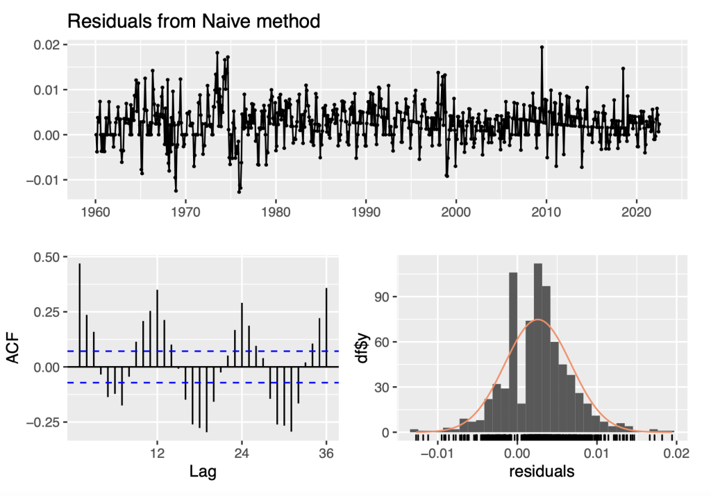

##
## Ljung-Box test
##
## data: Residuals from Naive method
## Q* = 812.21, df = 24, p-value < 2.2e-16
##
## Model df: 0. Total lags used: 24

The residuals from the Naive method look like white noise in terms of their variability being stable/constant over the analysis period and their distribution displayed in the histogram is reasonably close to a normal/Gaussian distribution. However, the ACF plot indicates that there is significant time dependence with high positive auto-correlations at lags 12, 24, and 36 and high negative auto-correlations at lags offset by 6 months prior.

f12 = forecast(Ylog_naive)
autoplot(Ylog_naive, include = 60)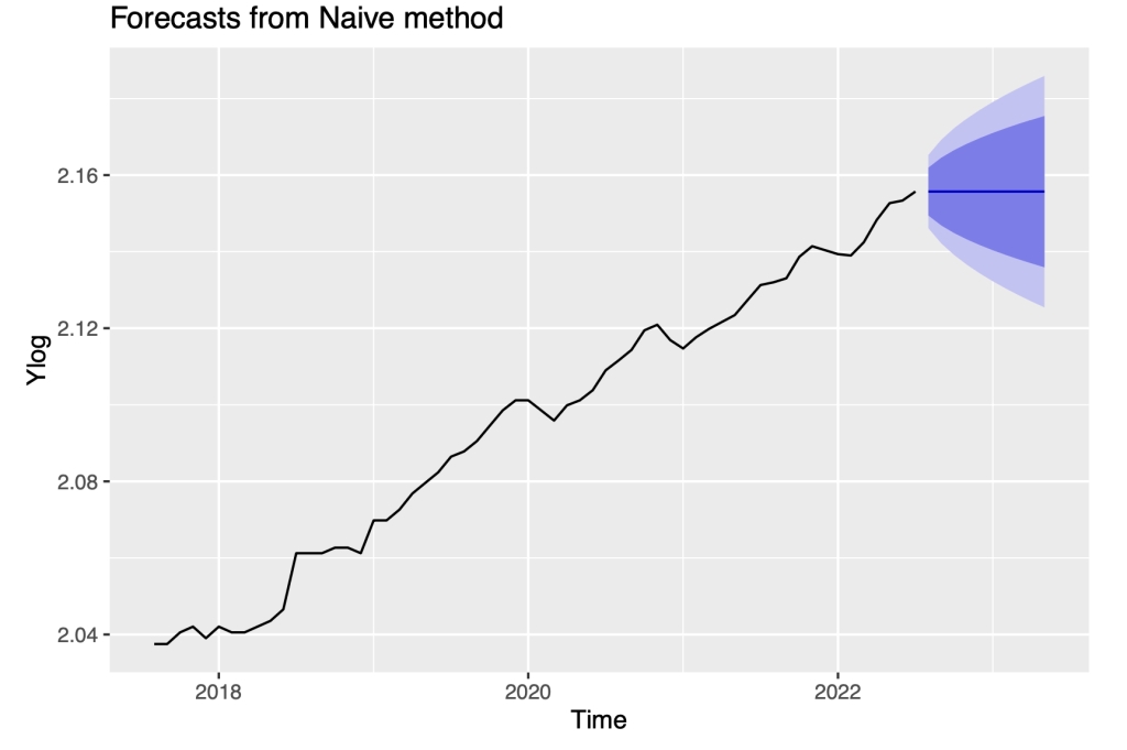

We repeat the computation of forecasts with the drift method. The Naive model does not exploit the strong auto-correlations in the forecast residuals. The forecast residuals are constant with the increasing width of the prediction intervals. Further analysis accommodating the time dependence in the residuals will be the focus of later sections.

4.3 Random Walk model with drift

The drift method is a slight variation of the Naive forecasting method. The drift methods allows the forecast to increase or decrease over a period of time. The amount of change over this time period is known as drift. The drift is set to be the average change seen in the data.

Ylog_rw <- rwf(Ylog, drift = TRUE) 
print(summary(Ylog_rw)) 

##
## Forecast method: Random walk with drift
##
## Model Information:
## Call: rwf(y = Ylog, drift = TRUE)
##
## Drift: 0.0026 (se 2e-04)
## Residual sd: 0.0042
##
## Error measures:
## ME RMSE
## Training set 2.986517e-17 0.004149668 0.003043804 -0.01635304 0.3998792
## MASE ACF1
## Training set 0.09321392 0.4691113
##
## Forecasts:
## Point Forecast Lo 80 Hi 80 Lo 95 Hi 95
## Aug 2022 2.158270 2.152949 2.163592 2.150132 2.166409
## Sep 2022 2.160845 2.153314 2.168375 2.149327 2.172362
## Oct 2022 2.163419 2.154189 2.172648 2.149303 2.177534
## Nov 2022 2.165993 2.155329 2.176657 2.149683 2.182303
## Dec 2022 2.168567 2.156636 2.180498 2.150320 2.186814
## Jan 2023 2.171141 2.158063 2.184220 2.151140 2.191143
## Feb 2023 2.173716 2.159580 2.187851 2.152097 2.195334
## Mar 2023 2.176290 2.161168 2.191411 2.153163 2.199416
## Apr 2023 2.178864 2.162814 2.194914 2.154318 2.203410
## May 2023 2.181438 2.164509 2.198367 2.155548 2.207329 MAE MPE MAPE

checkresiduals(Ylog_rw)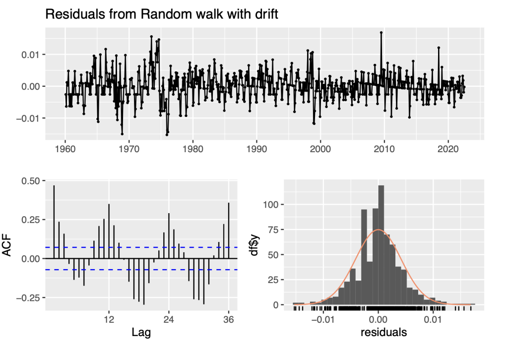 

##
## Ljung-Box test
##
## data: Residuals from Random walk with drift
## Q* = 812.21, df = 23, p-value < 2.2e-16
##
## Model df: 1. Total lags used: 24

The residuals from the Naive method look like white noise in terms of their variability being stable/constant over the analysis period and their distribution displayed in the histogram is reasonably close to a nor- mal/Gaussian distribution. However, the ACF plot indicates that there is significant time dependence with high positive auto-correlations at lags 12, 24, and 36 and high negative auto-correlations at lags offset by 6 months prior.

f12 = forecast(Ylog_rw)
autoplot(f12, include = 60)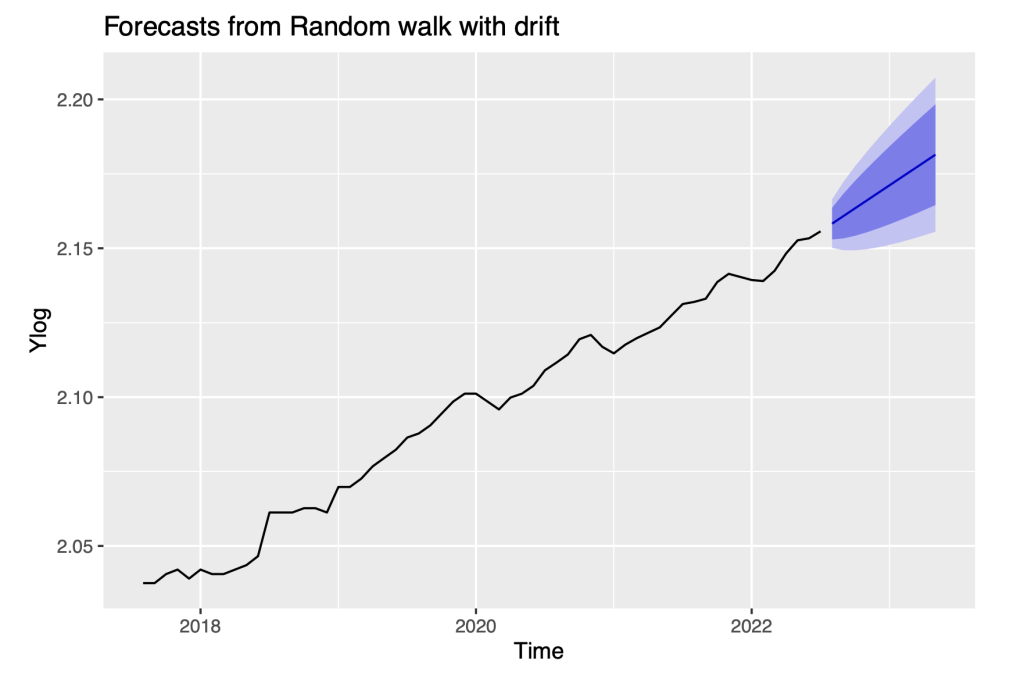

We repeat the computation of forecasts with this method. The random walk with drift model does forecast an upward trend in the series, but further analysis accommodating the time dependence in the residuals will be the focus of later sections.

So far, we can conclude:

• Transforming to log scale stabilizes the volatility of the series
• Extending the naive model to the random walk model with a positive drift captures the positive trend in the series.

Nonetheless, the residuals check of the random walk model indicates significant time dependence remains which we address with the development of Arima models below.

5. Non-stationary to Stationary

In the prior section, we explored the naive and random walk models for the log series which treat the original series as non-stationary but the first differences as stationary.

In this section we formally evaluate the stationarity or non-stationarity of the original log series and its series of first differences. We apply two tests, the ADF and KPSS tests. We begin with an overview of these two tests.

5.1 Understanding the ADF and KPSS Tests

Augmented Dickey Fuller (“ADF”) test and Kwiatkowski-Phillips-Schmidt-Shin (“KPSS”) test are two sta- tistical tests that are used to check the stationarity of a time series.[2]

Augmented Dickey Fuller (“ADF”) belongs to the ‘Unit Root test’. This is a method to test the stationarity of a time series. ADF is a statistical significant text. This implies a hypothesis testing is involved with a null and alternate hypothesis. As a result of hypothesis testing, a test statistic is computed and p-values get reported. Unit root is a characteristic of time series that makes it non-stationary.

• Null Hypothesis: The series has a unit root.
• Alternate Hypothesis: The series has no unit root.

A time series is consistent with having a unit root if the auto-regressive model of order p = 1 has auto- regressive parameter α1 = 1. Such a model corresponds to a random walk model which is non-stationary. The AR(1) model for a time series {yt} is given by:

yt = α0 + α1yt−1 + εt

where α0 and α1 are the constant model parameters and {εt} is the time series of errors in the model, assumed to be white noise.

Kwiatkowski-Phillips-Schmidt-Shin (“KPSS”) helps to determine if a time series is stationary around a mean or linear trend. A series will be non-stationary due to a unit root. Stationary time series is where the properties such as mean, variance and covariance are constant over time.

• The null hypothesis for the test is that the data is stationary.
• The alternate hypothesis for the test is that the data is not stationary.

KPSS test for stationarity of a series round a deterministic trends. Deterministic indicates that the slope of the trend does not change permanently. The test may not necessarily reject the null hypothesis (that the series is stationary) even if a series is steadily increasing or decreasing.[3]

Apply both tests to evaluate whether the (possibly de-trended) time series is consistent with being stationary. Possible conditions are given below:
Case 1: Both tests provide evidence that the series is not stationary – The series is not stationary.
Case 2: Both tests conclude that the series is stationary – The series is stationary.
Case 3: KPSS indicates stationarity and ADF indicates non-stationarity – The series is trend stationary. Trend needs to be removed to make series strict stationary. The detrended series is checked for stationarity.[2]
Case 4: KPSS indicates non-stationarity and ADF indicates stationarity – The series is difference stationary. Differencing is to be used to make series stationary. The differenced series is checked for stationarity.[2]

The table explains the conditions for a time series to be stationary based on the ADF and KPSS test.

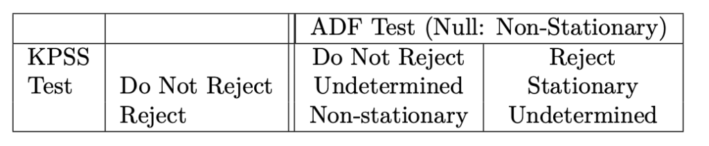
For a given time series to be stationary,

p-value of ADF < 0.05
p-value of KPSS > 0.05

5.2 Applying the tests to the log series

adf.test(Ylog) 

##
## Augmented Dickey-Fuller Test
##
## data: Ylog
## Dickey-Fuller = -2.2066, Lag order = 9, p-value = 0.4909
## alternative hypothesis: stationary

kpss.test(Ylog) 

## Warning in kpss.test(Ylog): p-value smaller than printed p-value

##
## KPSS Test for Level Stationarity
##
## data: Ylog
## KPSS Level = 10.846, Truncation lag parameter = 6, p-value = 0.01

The p-value of the ADF test is greater than 0.05 so the null hypothesis of non-stationarity is not rejected. The p-value of the KPSS test is less than 0.05 so the null hypothesis of can be rejected. Together these tests support the conclusion that the log series is non-stationary.

5.3 Methods to convert non-stationary to stationary

5.3.1 Differencing

Differencing is the process of transforming the time series. This can be used to remove the series dependence on time. Differencing can help stabilize the mean of the time series by removing changes in the level of a time series, and so eliminating (or reducing) trend and seasonality. This is one of the simplest method to convert non-stationary to stationary. This method calculates the difference between consecutive observations.[4]

ydi f f_t = y_t − y_t−1

We note that the naive and random walk models of the previous section explicitly model the differenced series as independent and identically distributed noise with either zero or non-zero mean. We now apply the ADF and KPSS tests to the differenced log series.

Apply the ADF and KPSS tests

Ylog_diff = diff(Ylog) 
plot(Ylog_diff)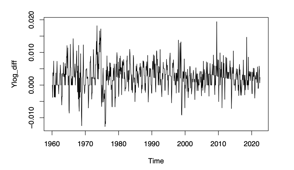

Apply the tests

adf.test(Ylog_diff) 

## Warning in adf.test(Ylog_diff): p-value smaller than printed p-value
##
## Augmented Dickey-Fuller Test
##
## data: Ylog_diff
## Dickey-Fuller = -6.4573, Lag order = 9, p-value = 0.01
## alternative hypothesis: stationary

kpss.test(Ylog_diff) 

## Warning in kpss.test(Ylog_diff): p-value greater than printed p-value
##
## KPSS Test for Level Stationarity
##
## data: Ylog_diff
## KPSS Level = 0.090151, Truncation lag parameter = 6, p-value = 0.1

The p-value of the ADF test is less than 0.05. The p-value of the KPSS tests is greater than 0.05. This satisfies the condition for stationarity. Therefore, we can proceed to develop stationary time series models on the differenced log series.

6. ARIMA Modeling of the Log CPI Series

6.1 ACF and PACF of the Differenced Series

To anticipate the development of time series models, we plot the ACF and PACF functions of the differenced log series.

ggAcf(Ylog_diff)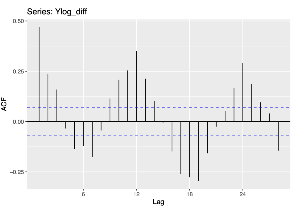

ggPacf(Ylog_diff)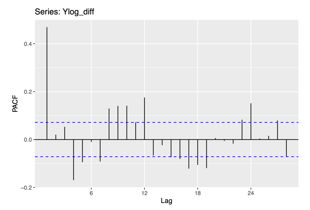

These are the same plots as given above in checking the residuals to the Naive method. Now, these suggest modeling the first differences with ARMA models.

6.2 ARIMA Models

ARIMA is the abbreviation for Auto-regressive Integrated Moving Average. It is the generalised version of the ARMA (Autoegressive moving average) model. Auto Regressive (AR) terms refer to the lags of the differenced series, Moving Average (MA) terms refer to the lags of errors and I is the number of difference used to make the time series stationary. Any ‘non-seasonal’ time series that exhibits patterns and is not a random white noise can be modeled with ARIMA models. While the random walk model suggests sea- sonal auto-correlations, we fit the ARIMA model with no seasonal terms first and consider seasonal models subsequently.[5][6]

An ARIMA model is characterized by 3 terms: p, d, q where,

• p is the order of the AR term
• q is the order of the MA term
• d is the number of differences required to make the time series stationary

fit_arima <- auto.arima(Ylog, seasonal = FALSE)
print(summary(fit_arima))

## Series: Ylog
## ARIMA(1,1,0) with drift
##
## Coefficients:
## ar1 drift
## 0.4688 0.0026
## s.e. 0.0322 0.0003
##
## sigma^2 = 1.346e-05: log likelihood = 3142.48
## AIC=-6278.95 AICc=-6278.92 BIC=-6265.09
##
## Training set error measures:
## ME RMSE MAE
## Training set 2.61495e-07 0.003662036 0.002756685 -0.007444624 0.3553743
## MASE ACF1
## Training set 0.08442116 -0.009434406

checkresiduals(fit_arima)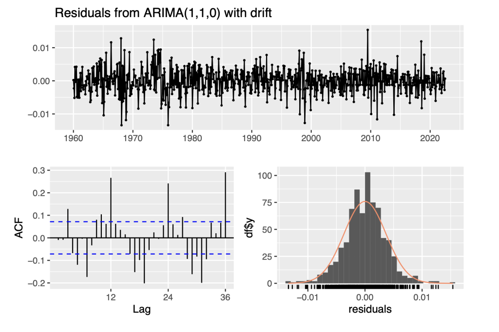

##
## Ljung-Box test
##
## data: Residuals from ARIMA(1,1,0) with drift
## Q* = 236.24, df = 23, p-value < 2.2e-16
##
## Model df: 1. Total lags used: 24

The R function auto.arima selects the ARIMA(1,1,0) model which corresponds to a first-order auto-regression model of the differenced log series. Using the notation

yt = Ylogt −Ylogt−1
yˆ t = αˆ 0 + αˆ 1 y t − 1

Where
αˆ0 = 0.00257
αˆ0 is the drift.
and
αˆ1 = 0.4688

The analysis of residuals from this model indicates significant time dependence that appears to be seasonal, with high auto-correlations at lags 12, 24, 36. We thus pursue seasonal ARIMA models in the next section.

fit_arima$coef 

## ar1 drift
## 0.46879585 0.00257475

Implement forecast methods for interval h = 12

f12 = forecast(fit_arima,h = 12)
autoplot(f12,include = 60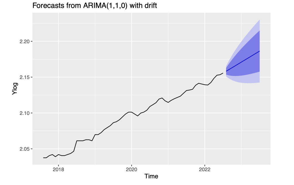

6.3 Seasonal ARIMA Models

Seasonal Auto-regressive Integrated Moving Average, or SARIMA, method for time series forecasting with univariate data containing trends and seasonality.[7] This model combines both non-seasonal and seasonal components in a multiplicative model. The seasonal ARIMA model is implemented to accommodate the seasonal pattern present in the time series. The shorthand notation for Seasonal ARIMA is

ARIMA(p,d,q)×(P,D,Q)[m] [8]

where,

• P = seasonal AR order,
• D = seasonal difference order,
• Q = seasonal MA order,
• m = number of observations per year.

6.4 Fitting Seasonal Arima model to the entire time series

We apply the auto.arima model on the logarithm transform of the original series. We set seasonal equal to TRUE, since seasonality is present in the time series.

fit_sarima<- auto.arima(Ylog, seasonal = TRUE) 
print(fit_sarima) 

## Series: Ylog
## ARIMA(5,0,0)(2,1,0)[12] with drift
##
## Coefficients:
## ar1 ar2 ar3 ar4 ar5 sar1 sar2
## 1.3294 -0.3364 0.1218 -0.0642 -0.067 -0.6580 -0.3734 0.0025
## s.e. 0.0367 0.0615 0.0630 0.0616 0.037 0.0347 0.0342 0.0003
##
## sigma^2 = 1.245e-05: log likelihood = 3123.34
## AIC=-6228.69 AICc=-6228.44 BIC=-6187.24

checkresiduals(fit_sarima)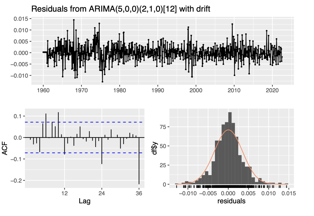 

##
## Ljung-Box test
##
## data: Residuals from ARIMA(5,0,0)(2,1,0)[12] with drift
## Q* = 58.295, df = 17, p-value = 2.003e-06
##
## Model df: 7. Total lags used: 24

To evaluate the robustness of the auto.arima function with seasonal models, we also apply the function to the differenced series.

Ylog_diff0<- na.omit(diff(Ylog)) 
fit_sarima<- auto.arima(Ylog_diff0, seasonal = TRUE)
print(fit_sarima)

## Series: Ylog_diff0
## ARIMA(1,0,0)(2,0,0)[12] with non-zero mean
##
## Coefficients:
## ar1 sar1 sar2 mean
## 0.4207 0.2256 0.1867 0.0025
## s.e. 0.0334 0.0361 0.0359 0.0004
##
## sigma^2 = 1.204e-05: log likelihood = 3184.54
## AIC=-6359.09 AICc=-6359.01 BIC=-6335.99

checkresiduals(fit_sarima)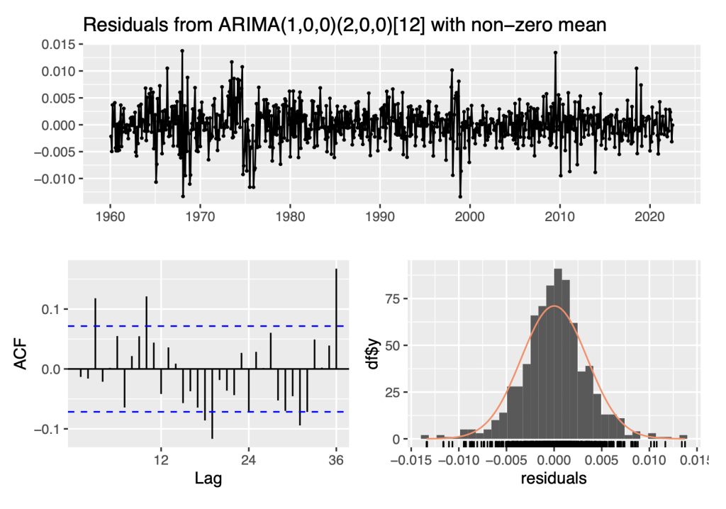

##
## Ljung-Box test
##
## data: Residuals from ARIMA(1,0,0)(2,0,0)[12] with non-zero mean
## Q* = 64.569, df = 21, p-value = 2.538e-06
##
## Model df: 3. Total lags used: 24

This second fitted model is less complex than the first in terms of having fewer parameters However, the residual analysis indicates that that the residual time series is not consistent with white noise.

To resolve this issue we will fit SARIMA models to shorter time series and evaluate their goodness-of-fit in terms of the p-values of the Ljung-Box test of the model residuals.

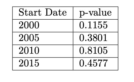
6.5 Fitting Sarima models to shorter analysis periods

The time series is divided into 4 sub series, each with a different start date. The 4 series start from the year 2000, 2005, 2010 and 2015. All the 4 time series end at the December of 2018. Based on the available time series, we forecast for the year 2019. Due to the recent COVID-19 pandemic, the forecasting model may not be accurate due to the sudden halt of the world’s economy in the year 2020. Therefore, we will forecast for the year 2019.

6.5.1 Start date set as January 2000

For this time series, the start date is set as the month of January, in the year 2000.

Ylog_diff0<- na.omit(diff(Ylog)) 
Ylog_diff1<- window(Ylog_diff0, start=c(2000,1), end = c(2018,12))
fit_sarima1<- auto.arima(Ylog_diff1, seasonal = TRUE)
print(fit_sarima1)

## Series: Ylog_diff1
## ARIMA(0,0,1)(2,0,0)[12] with non-zero mean
##
## Coefficients:
## ma1 sar1 sar2 mean
## 0.2092 0.3579 0.2742 0.0021
## s.e. 0.0670 0.0638 0.0652 0.0005
##
## sigma^2 = 7.346e-06: log likelihood = 1023.51
## AIC=-2037.02 AICc=-2036.74 BIC=-2019.87

checkresiduals(fit_sarima1)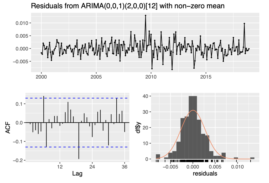

##
## Ljung-Box test
##
## data: Residuals from ARIMA(0,0,1)(2,0,0)[12] with non-zero mean
## Q* = 28.937, df = 21, p-value = 0.1155
##
## Model df: 3. Total lags used: 24

6.5.2 Start date set as January 2005

For this time series, the start date is set as the month of January, in the year 2005.

Ylog_diff0<- na.omit(diff(Ylog)) 
Ylog_diff1<- window(Ylog_diff0, start=c(2005,1), end = c(2018,12)) fit_sarima2<- auto.arima(Ylog_diff1, seasonal = TRUE) print(fit_sarima2) 

## Series: Ylog_diff1
## ARIMA(0,0,1)(2,0,0)[12] with non-zero mean
##
## Coefficients:
## ma1 sar1 sar2 mean
## 0.1999 0.3580 0.2420 0.0024
## s.e. 0.0780 0.0758 0.0777 0.0006
##
## sigma^2 = 8.78e-06: log likelihood = 739.4
## AIC=-1468.8 AICc=-1468.43 BIC=-1453.18 checkresiduals(fit_sarima2)

##
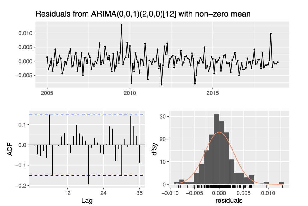
## Ljung-Box test
##
## data: Residuals from ARIMA(0,0,1)(2,0,0)[12] with non-zero mean
## Q* = 22.341, df = 21, p-value = 0.3801
##
## Model df: 3. Total lags used: 24

6.5.3 Start date set as January 2010

For this time series, the start date is set as the month of January, in the year 2010

Ylog_diff0<- na.omit(diff(Ylog)) 
Ylog_diff1<- window(Ylog_diff0, start=c(2010,1), end = c(2018,12)) fit_sarima3<- auto.arima(Ylog_diff1, seasonal = TRUE) print(fit_sarima3) 

## Series: Ylog_diff1
## ARIMA(0,0,1)(2,0,0)[12] with non-zero mean
##
## Coefficients:
## ma1 sar1 sar2 mean
## 0.1888 0.3659 0.3518 0.0023
## s.e. 0.0970 0.0921 0.1029 0.0008 ##
## sigma^2 = 7.916e-06: log likelihood = 479.2
## AIC=-948.4 AICc=-947.82 BIC=-934.99

checkresiduals(fit_sarima3)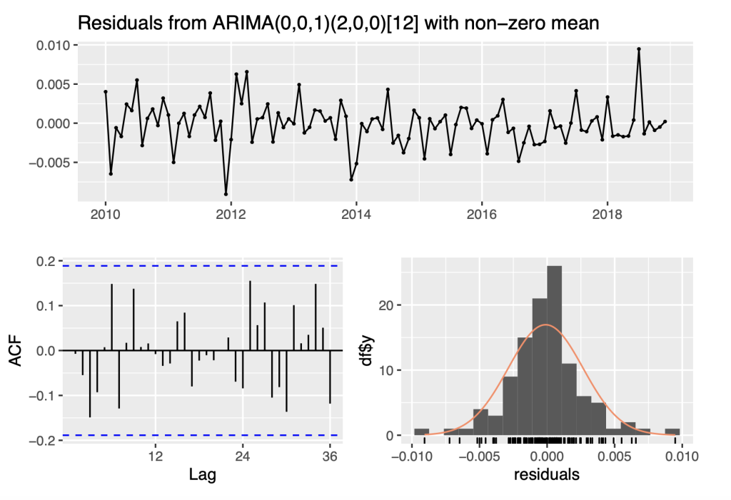

##
## Ljung-Box test
##
## data: Residuals from ARIMA(0,0,1)(2,0,0)[12] with non-zero mean
## Q* = 13.528, df = 19, p-value = 0.8105
##
## Model df: 3. Total lags used: 22

6.5.4 Start date set as January 2015

For this time series, the start date is set as the month of January, in the year 2015.

Ylog_diff0<- na.omit(diff(Ylog))
Ylog_diff1<- window(Ylog_diff0, start=c(2015,1), end = c(2018,12))
fit_sarima4<- auto.arima(Ylog_diff1, seasonal = TRUE)
print(fit_sarima4)

## Series: Ylog_diff1

## ARIMA(0,0,0)(0,1,0)[12]
##
## sigma^2 = 6.88e-06: log likelihood = 162.88
## AIC=-323.76 AICc=-323.65 BIC=-322.18

checkresiduals(fit_sarima4)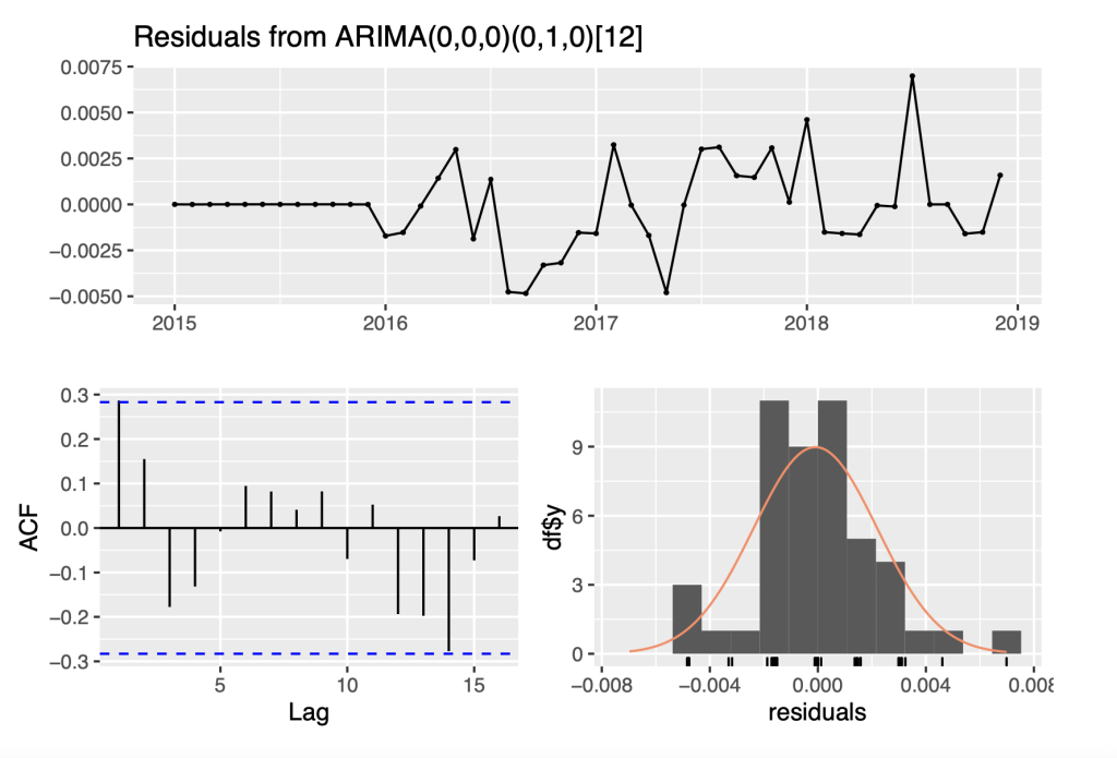

##
## Ljung-Box test
##
## data: Residuals from ARIMA(0,0,0)(0,1,0)[12]
## Q* = 9.8053, df = 10, p-value = 0.4577
##
## Model df: 0. Total lags used: 10

fs1 = forecast(fit_sarima1,h = 12)
fs2 = forecast(fit_sarima2,h = 12)
fs3 = forecast(fit_sarima3,h = 12)
fs4 = forecast(fit_sarima4, h = 12)
Ylog_diff <- window(Ylog_diff0,start = c(2018,1),end = c(2018,12))
Ylog_forecast <- window(Ylog_diff0, start = c(2019,1), end = c(2019,12))
autoplot(Ylog_diff) +
  autolayer(Ylog_forecast, series = "Original") +
  autolayer(fs1, series = "Start Date: 2000", PI = FALSE) +
  autolayer(fs2, series = "Start Date: 2005", PI = FALSE) +
  autolayer(fs3, series = "Start Date: 2010", PI = FALSE) +
  autolayer(fs4, series = "Start Date: 2015", PI = FALSE) +
  xlab("Year") + ylab("CPI") +
  labs(title = "Forecasts of various Models")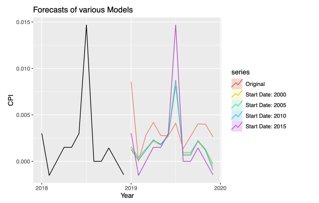

df_fs1 = as.data.frame(fs1)
df_fs2 = as.data.frame(fs2)
df_fs3 = as.data.frame(fs3)
df_fs4 = as.data.frame(fs4)
df_val1 = df_fs1$'Point Forecast'
df_val2 = df_fs2$'Point Forecast'
df_val3 = df_fs3$'Point Forecast'
df_val4 = df_fs4$'Point Forecast'
df_val1

## [1] 0.0013946373 0.0002292368 0.0012037319 0.0021735141 0.0017378107
## [6] 0.0026955593 0.0081294351 0.0007698798 0.0007698798 0.0021182348
## [11] 0.0011841142 -0.0005755733

tab <- matrix(NA,ncol=2,nrow=4)
tab[1,1] <- rmse(df_val1, Ylog_forecast)
tab[2,1] <- rmse(df_val2, Ylog_forecast)
tab[3,1] <- rmse(df_val3, Ylog_forecast)
tab[4,1] <- rmse(df_val4, Ylog_forecast)
tab[1,2] <- mad(df_val1 - Ylog_forecast)
tab[2,2] <- mad(df_val2 - Ylog_forecast)
tab[3,2] <- mad(df_val3 - Ylog_forecast)
tab[4,2] <- mad(df_val4 - Ylog_forecast)
colnames(tab) <- c("RMSE","MAE")
rownames(tab) <- c("2000","2005","2010","2015")
knitr::kable(tab)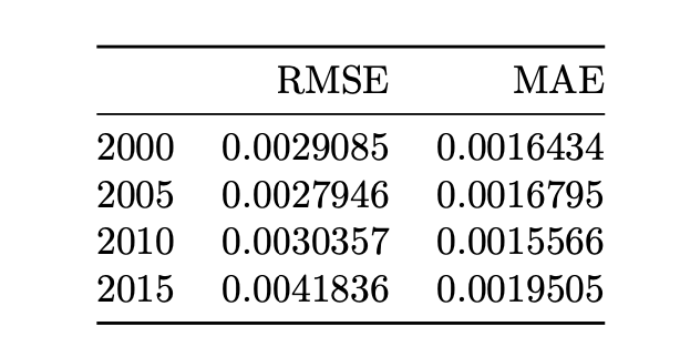

# Plot time series of forecast errors
#df_ferror<- rbind(

tmp<-
  rbind(data.frame(

    Date = as.numeric(time(Ylog_forecast)),
    Error =as.numeric(df_val1 - Ylog_forecast),
    StartDate="2000"),
    data.frame(
    Date = as.numeric(time(Ylog_forecast)),
    Error =as.numeric(df_val2 - Ylog_forecast),
    StartDate="2005"),
    data.frame(
    Date = as.numeric(time(Ylog_forecast)),
    Error =as.numeric(df_val3 - Ylog_forecast),
    StartDate="2010"),
    data.frame(
    Date = as.numeric(time(Ylog_forecast)),
    Error =as.numeric(df_val4 - Ylog_forecast),
    StartDate="2015")

  )
ggplot(tmp, aes(x=Date,y=Error, col=StartDate)) + geom_line()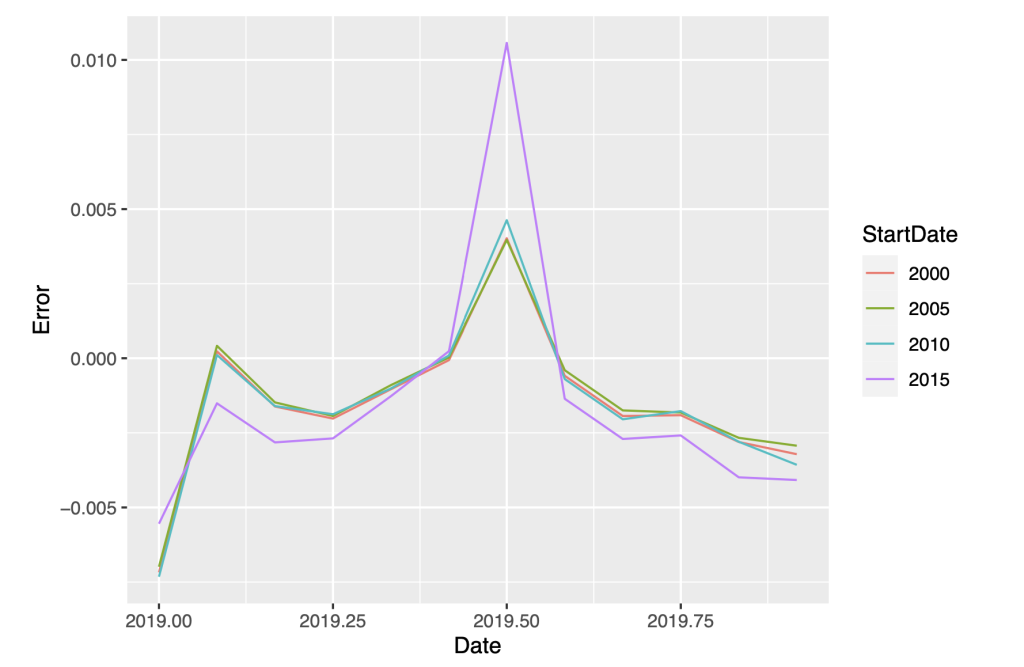

The forecasts with start dates 2000, 2005, and 2010 are nearly indistinguishable, and their accuracy statistics are comparable and smaller than the start date of 2015. We conclude that the forecast model with start date of 2000 is the preferred model because of its high degree of accuracy and stability over the specification with shorter training periods.

In conclusion, we present the summary of this model and its forecasts for the India CPI.

7.References

[1] https://www.jatinverma.org/retail-inflation-eases-to-658-industrial-production-quickens
[2] https://www.statsmodels.org/dev/examples/notebooks/generated/stationarity_detrending_adf_kpss.html
[3] https://www.machinelearningplus.com/time-series/kpss-test-for-stationarity/
[4] https://norman-restaurant.com/what-does-differencing-mean-in-time-series/
[5] https://datascienceplus.com/time-series-analysis-using-arima-model-in-r/
[6] https://otexts.com/fpp2/arima-r.html
[7] https://machinelearningmastery.com/sarima-for-time-series-forecasting-in-python/ [8] https://online.stat.psu.edu/stat510/lesson/4/4.1

---