

Author: Adarsh Sasikumar
Mentor: Dr. Hong Pan
Sri Kumaran Children’s Home of Educational Council
Abstract
While there is a burgeoning research literature on crime trends, much of the extant research has adopted a relatively narrow approach, efforts across studies are highly variable. In this paper, we outline a method to establish the relation between crime rate in the two years of 1959 and 1960 to the political, social and economic factors of that time, whether the crime does depend on the poverty state and mindset of the people in that era. The correlation between crime rate and all the factors being studied is visualized using a scatterplot matrix (SPLOM). Multiple linear regression models under ANOVA framework are performed to evaluate which factors and their interactions affect the crime rates significantly. Hence, what should be done in order to reduce the crime rate and help in the development of the country in all aspects. Statistically, the factors which influence crime rate the most are police expenditure in both the years, Gross Domestic Product (GDP), State population and probability of imprisonment.
I. Introduction
A. Background
Crime is an illegal act which is subjectable to punishment by the government. It involves violating the standard law code prescribed by a country’s parliament and judiciary. It is an unlawful act and a grave offense against human morality. The topic covered in this paper is the data analysis of crimes in the United States. It is a systematic way of detecting and investigating patterns and trends in crime.
The crime in the U.S. has been recorded since the early 1600s. The crime rates have varied over time, with a sharp rise after 1900 and reaching a broad bulging peak between the 1970s and early 1990s. The range of these criminal activities vary from pickpocketing to serial killing and assassinations. The basic aspect of a crime considers the offender, the victim, type of crime, severity and level, and location. These are the basic questions asked by law enforcement when investigating any situation. This information is formatted into a government record by a police arrest report, also known as an incident report.
Society has a strong misconception about crime rates due to media aspects heightening their fear factor. The manner, in which America’s crime rate compared to other countries of similar wealth and development depends on the nature of the crime used in the comparison. Overall crime statistic comparisons are difficult to conduct, as the definition and categorization of crimes varies across countries. Thus, an agency in a foreign country may include crimes in its annual reports which the United States omits, and vice versa. However, some countries such as Canada have similar definitions of what constitutes a violent crime as America. Overall, the total crime rate is more in the US than it is in other developed countries across Europe.
B. Problem Statement
The criminal behaviour has traditionally been linked to the offender’s presumed unique motivation which might be various factors such as unemployment, family circumstances due to poverty. It also depends on the dark figure of crime which is the gap between reported and unreported crimes calls the reliability of an official crime statistics into question, but all measures of crime have a dark figure to some degree. The gap in official statistics is largest for less serious crimes. It also varies from region to region or as a matter of fact, state to state. It depends on the type of community living in that region as well. The crime in metropolitan statistical areas tends to be above the national average; however, wide variance exists among and within metropolitan areas.
In this report, we will deep dive into various factors contributing/influencing the rate of crime, which serves as our dependent variable and how it depends on 15 independent variables, which are: % of males aged 14–24, indicator variables for a Southern state, mean years of schooling, police expenditure in 1960 and 1959, labour force participation rate, number of males per 1000 females, state population, number of non- whites per 1000 people, unemployment rate of urban males age 14–24 & 35–39, gross domestic product per head, income inequality, probability of imprisonment, and average time served in state prisons, that affect the rate of crime in a specific category per head population.
II. Methodology
A. Descriptive
In this section, we are going to describe, explore and confirm how the economic, social and political factors are affecting the crime rate using the MASS Library in R.
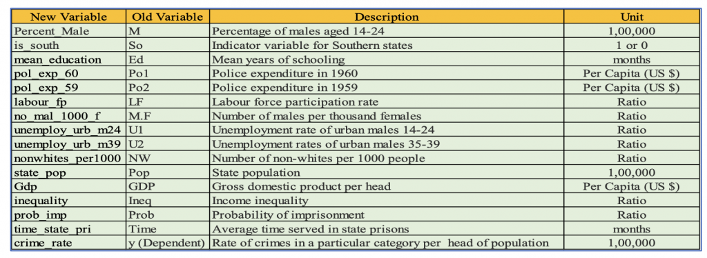
Table 1 : Variables used in this Model
Each row represents a state in the USA and Unit are shown in Table 1.
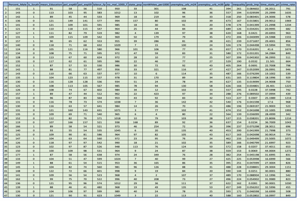
Table 2 : Crime Dataset
The rate of crime serves as the dependent variable which depends on a number of independent variables such as police expenditure, mean year of schooling, unemployment rate, income inequality, imprisonment probability and so on.
A SPLOM plot is used to show the basic information of the dataset. It is a collection of scatter plots being organized into matrix. It gives us the direction, strength, and linearity of the relationship between the dependent and independent variables and also helps in determining the correlation between the independent variable and dependent variable as seen in the Figure 1.
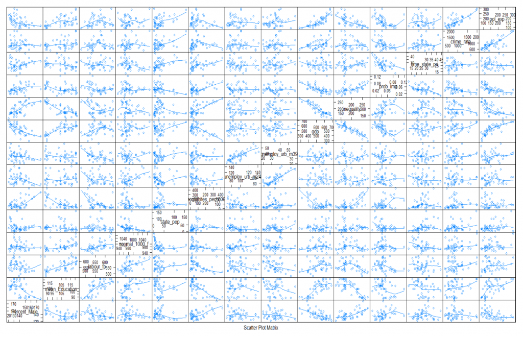
Figure 1 : SPLOM Plot with All Variables
B. Exploratory:
The data is first explored and wrangled to check for the presence of outliers and those which are present are removed.
The potential correlation between the variables is further evaluated via analysis by 14 simple regression models, to examine which independent variables are significant factors. Based on this set of simple regression models, 4 variables are chosen which have a statistically significant correlations with the dependent variable Crime Rate.
Regression is used to predict a continuous outcome based on one or more continuous predictor variables. Regression line is the straight line passing through the data that minimizes the sum of the squared differences between the original data and the fitted points.
An aov (analysis of variance) model is performed to check the interrelation between the 4 independent variables from the simple regression model. This analysis is performed iteratively on the various combinations in which the least significant combination (the one with highest p value) is removed after each step. Multiple regression analysis is performed on these 4 independent variables with respect to the dependant variable that is crime rate.
C. Confirmatory:
ANOVA model is used for deciding the best multiple regression model among the given combination of the 4 independent variables. ANOVA and step aic are used to find out the interdependency between the 4 variables. Likelihood ratio test is performed to check goodness of the fit of the nested regression models.
ANOVA is fundamental for all statistical approaches. ANOVA, which stands for Analysis of Variance, is a statistical test used to analyses the difference between the means of more than two groups.
ANOVA is used in the analysis of comparative experiments, those in which only the difference in outcomes is of interest. The statistical significance of the experiment is determined by a ratio of two variances. This ratio is independent of several possible alterations to the experimental observations: Adding a constant to all observations does not alter significance. Multiplying all observations by a constant does not alter significance.
A one-way ANOVA uses one independent variable, while a two-way ANOVA uses two independent variables.
In ANOVA, the null hypothesis is that there is no difference among group means. If any group differs significantly from the overall group mean, then the ANOVA will report a statistically significant result.
So, ANOVA statistical significance result is independent of constant bias and scaling errors as well as the units used in expressing observations. This makes it the ideal model.
We use ANOVA, when we want to test a hypothesis. From our 3 models of different combinations, we choose the model (independent variables) with maximum influence on the dependent variable that is crime rate as an ideal model. Finally, the model with all 4 variables is plotted. Following this, the best model is chosen from all the 3 models.
The likelihood-ratio test compares the goodness of fit of two nested regression models based on the ratio of their likelihoods, specifically one obtained by maximization over the entire parameter space and another obtained after imposing some constraint. A nested model is simply a subset of the predictor variables in the overall regression model.
III. Results
A. Descriptive
In this section, we will be depicting the various results of our analysis of regression and ANOVA Models.
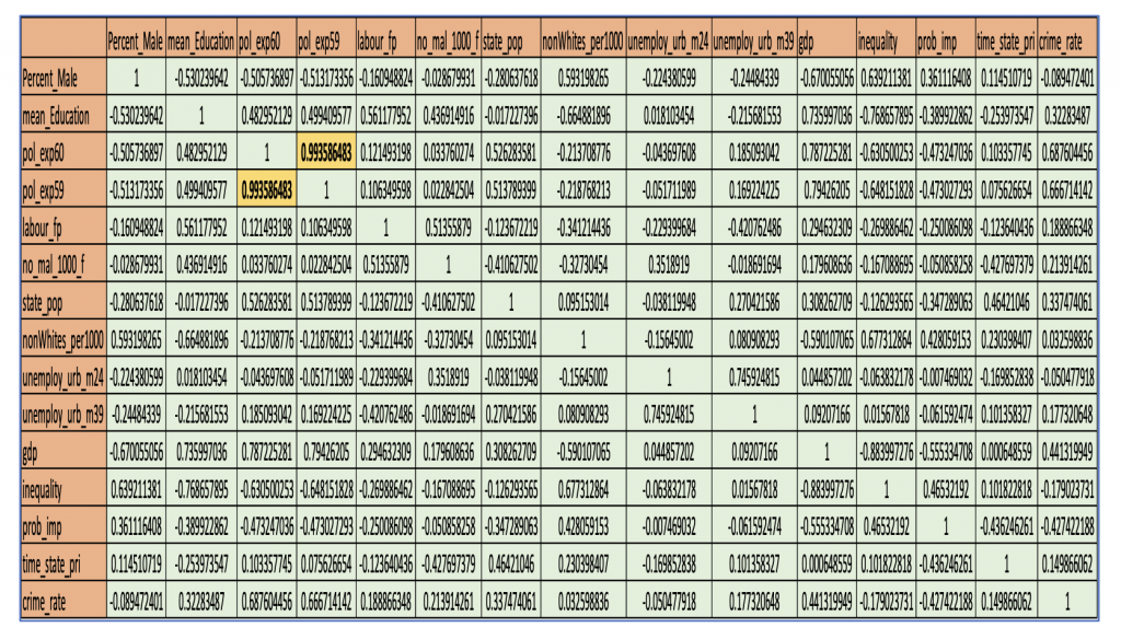
From Figure 2, we can see that police expenditure in 1959 and 1960 have high correlation with one another. This condition is not ideal for linear regression because no predictor variable should strongly correlate with one another, hence we are combining both into a single variable.
SPLOM PLOT
As we can see for police expenditure, state population and gdp vs Crime Rate from Figure 3, the data points are closer to the line moving in the upward direction indicating a strong positive linear relationship with crime rate. Similarly, for probability of imprisonment, it is in the downward direction indicating a strong negative relationship with Crime Rate.
From the plot, we can see that four independent variables with most correlation with the Crime Rate is Police expenditure, GDP, Probability of imprisonment and State Population.
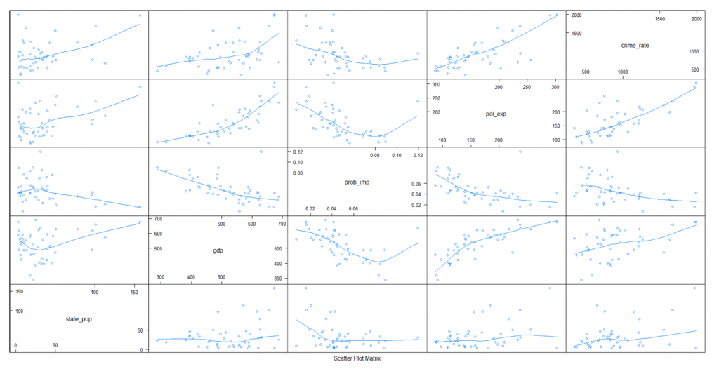
Figure 3 : SPLOM Plot with 4 Variables
B. Exploratory:
Data Wrangling
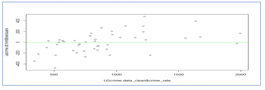
In Figure 4, the data is plotted with and without outlier.
The predictor variable during a simple linear regression must always have high linear relationships with target variables. So, for this data we need to first check for the presence of an outlier and if there are any, we must remove them.
If we look at the abline of the plot, we can see that the outliers of our data have a high influence over our model. Therefore, it is safer to remove the outliers from the data. The removal of outliers increases the R-squared of the model ~0.6 points, and the p value has decreased along with the value of intercept which shows the removal of outlier improves the model.
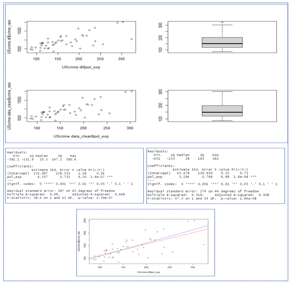
Figure 4 : Data Wrangling
A simple linear regression model is estimated for each of these 14 independent variables and their result has been tabulated below.
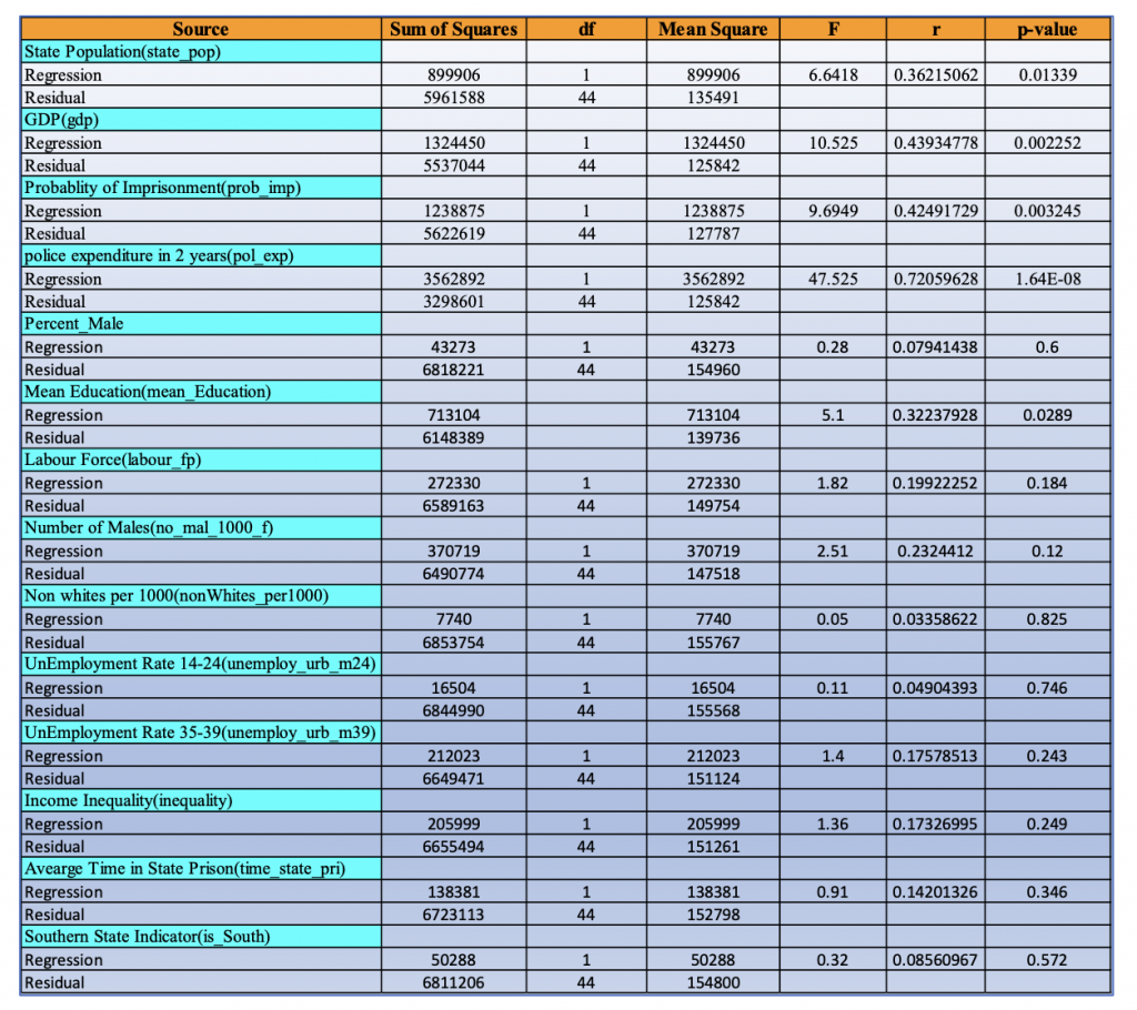
From these simple regression models, we can conclude that the relation between police expenditure, GDP, probability of imprisonment, state population and crime rate is highest as their p value is less than 0.05 with r being 72% ,44% ,43% and 36% respectively. So, with these 4 variables, a multiple regression and stepAIC is plotted. As next step, ANOVA is used to find the best model.
C. Confirmatory:
Interrelation between variables using multiple regression and stepAIC
AOV is performed to check which variables among the 4 variables have the most interrelation amongst one another and hence affect the crime rate.
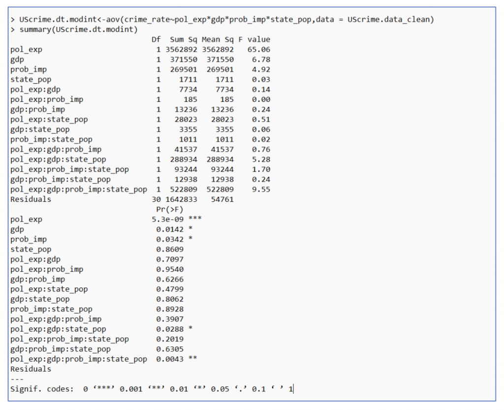
Figure 6 : Result of Interrelation – 4 Variables
Multiple regression and stepAIC are performed for the 4 interdependent variables as shown in Figure 7
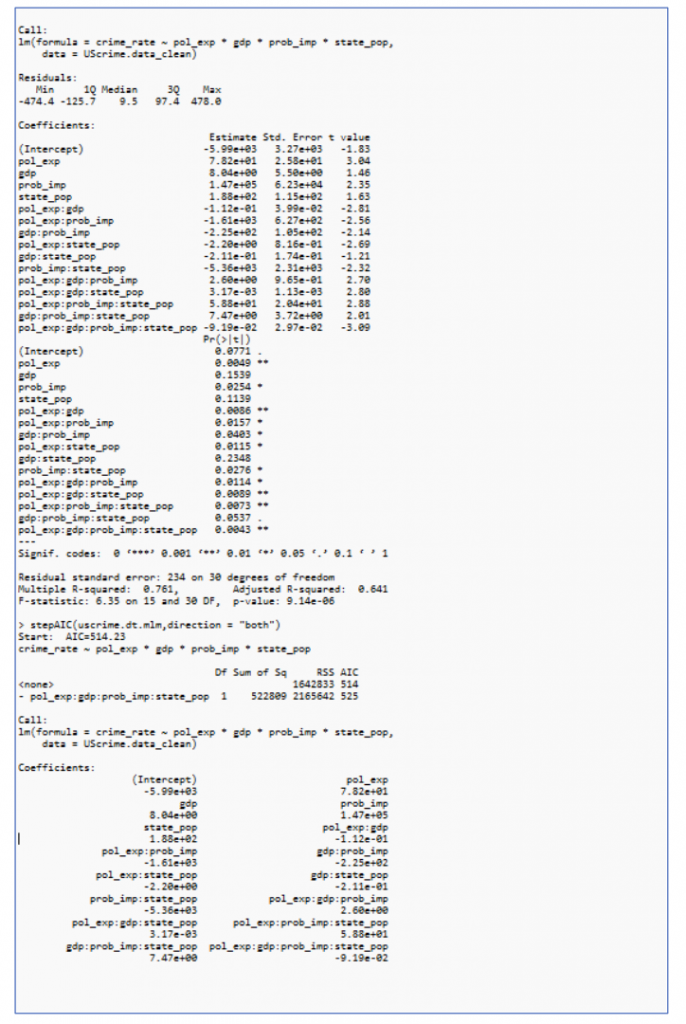
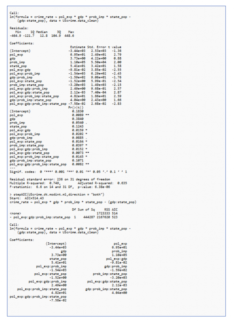
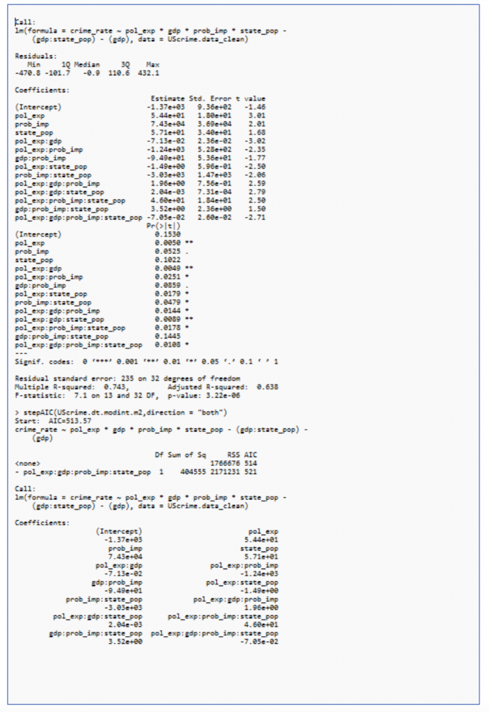
The highest p value (gdp:state_pop and gdp) are iteratively removed and performed multiple regression and stepAIC as shown in Figure 8 and 9
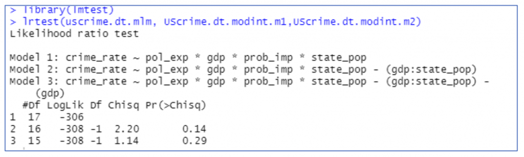
ANOVA is performed to check the best model.
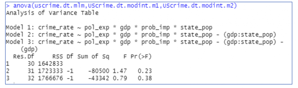
Figure 10 : ANOVA Model
ANOVA
Likelihood ratio test is performed on the 3 nested models, since the p value is greater than 0.05 as seen in the figure, we have to accept the null hypothesis which means there is not much difference between the models and the best fit is the first model (pol_exp * gdp * prob_imp * state_pop)
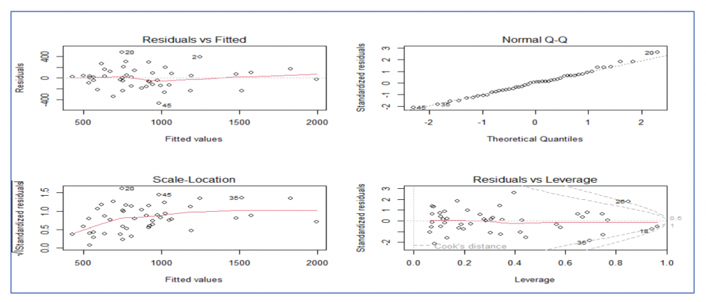
D. Model Validation
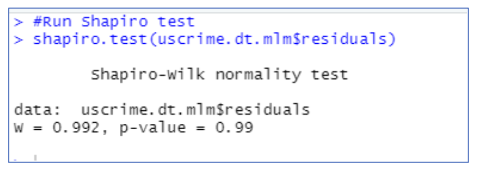
Figure 12 : Model Validation – Shapiro
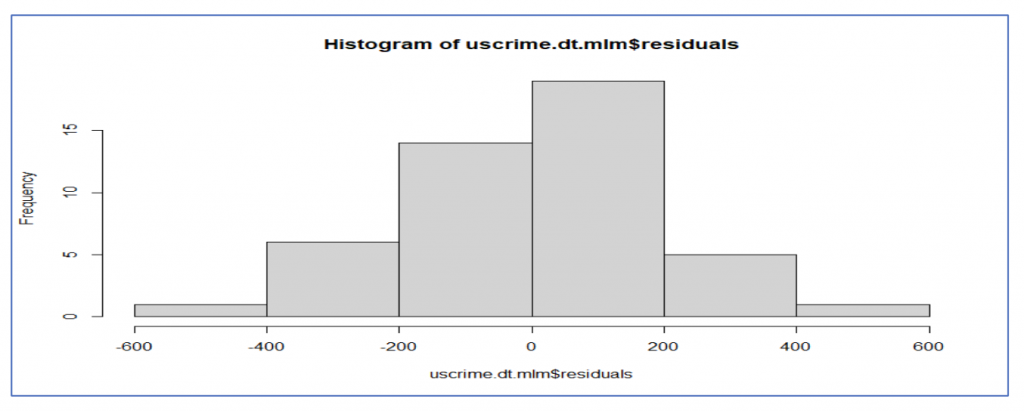
So, from the Shapiro test we can see that p value is more than 0.05 and hence confirms the data is normally distributed.
IV. Discussion
From the simple linear regression, multiple regression and ANOVA model, we can conclude that 4 factors which crime rate depends the most are police expenditure, GDP, State Population and probability of imprisonment.
Out of these 4 it depends on police expenditure the most followed by probability of imprisonment, which has a negative relation and then GDP followed by state population. From, the interrelation model, we can see how closely these 4 are interrelated and affect crime rate. As we can see the economic factors especially the police expenditure and the GDP which affected crime rate. Population factors also affected the crime rate as highly populated states experienced more crimes than the other states.
This was closely followed by putting fear into people’s mind by the probability of imprisonment playing a key role. It is an extremely surprising fact that crime rate is more influenced by the economic factors than unemployment.
Change in population in turn influences the gdp. The gdp of a state decides its expenditure on police. Despite the significant findings, there were several limitations to note in the study. The first limitation was the medium sample size.
V. Conclusion
From the simple linear regression, multiple regression and ANOVA model, we can conclude that 4 factors which crime rate depends the most are police expenditure, GDP, state population, and probability of imprisonment. Out of these 4 it depends on police expenditure the most followed by probability of imprisonment, which has a negative relation and then GDP followed by state population. From, the interrelation model, we can see how closely these 4 are interrelated and affect crime rate. As we can see the economic factors especially the police expenditure and the GDP which affected crime rate. Population factors also affected the crime rate as highly populated states experienced more crimes than the other states. This was closely followed by putting fear into people’s mind by the probability of imprisonment playing a key role. It is an extremely surprising fact that crime rate is more influenced by the economic factors than unemployment.
Change in population in turn influences the gdp. The gdp of a state decides its expenditure on police.
The state must allocate funds towards police training, enforce strict law & order and improves GDP by increasing Government spending, Export and Investment. This helps to bring down the crime rate.
VI. Reference list
- Venables, W. N. & Ripley, B. D., Modern Applied Statistics with S, Fourth edition (2003)
- Isaac Ehrlich, Participation in Illegitimate Activities: A Theoretical and Empirical Investigation (1973)
- Geoffrey R Norman and David L Streiner, BIOSTATISTICS: The Bare Essentials, Third Edition (2008)
- Adarsh S, GitHub Repository, https://github.com/AdarshS20/UScrimeDataAnalysis (2022)\
Acknowledgements
I would like to take this opportunity to express my profound gratitude and deep regards to my mentor Dr. Hong Pan for his exemplary guidance, monitoring and constant encouragement for this research paper. I would also like to take this opportunity to express my gratitude to Ms. Danielle Voorhies for her cordial support and guidance. Lastly, I thank my parents and friends for their encouragement and support to complete this research paper.
About the author
Adarsh Sasikumar
Adarsh is a 12th Grader at Sri Kumaran Children’s Home of Educational Council, Bangalore, India. He discovered the subject of Mathematics at the age of 6 and it was love at first sight. As he grew up, he felt like he had encapsulated himself into the number, angles, variables, and equations. He is planning to pursue an undergraduate major in Mathematics and is interested in predictive analysis.